Tom West Top Cutting

import geolime as geo
import seaborn as sns
import numpy as np

dh_tom = geo.read_file("../data/dh_tom_comp.geo")

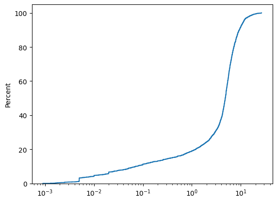
sns.ecdfplot(x=dh_tom["Zn_pct"], log_scale=True, stat='percent')

<Axes: ylabel='Percent'>

Using Numpy we can compute the coefficient of variation.

Note that we use the nanXXX function such as nanmean and nanstd to account the fact we have nan values in the array. If we were to use mean and std the results would be nan.

np.nanstd(dh_tom['Zn_pct']) / np.nanmean(dh_tom['Zn_pct'])

0.7653989945584244

np.nanmean(dh_tom['Zn_pct'])

4.901401374850275

The nan filter can also be made at the GeoLime level.

np.mean(dh_tom.data('Zn_pct', region="Zn_pct.notna()"))

4.901401374850275

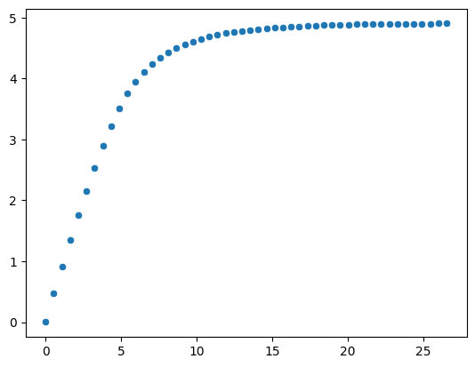
To analyse the different capping values, we can also perform a loop and compute the new mean after each capping.

We can create a range of 50 values between the minimum and the maximum values.

capped_mean = []
capped_values = np.linspace(
    start=np.nanmin(dh_tom['Zn_pct']), 
    stop=np.nanmax(dh_tom['Zn_pct']), 
    num=50
)
for cap in capped_values:
    zn_intermed = dh_tom['Zn_pct']
    zn_intermed[zn_intermed > cap] = cap
    capped_mean.append(np.nanmean(zn_intermed))

sns.scatterplot(x=capped_values, y=capped_mean)

<Axes: >

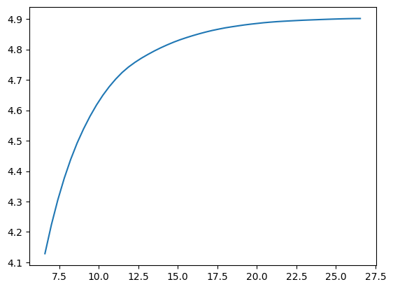
We can also create a linear spacing of 50 values between the 3rd quartile and the maximum of the value to zoom in in the most interesting part of the distribution.

capped_mean = []
capped_values = np.linspace(
    start=np.nanquantile(dh_tom['Zn_pct'], 0.75), 
    stop=np.nanmax(dh_tom['Zn_pct']), 
    num=50
)
for cap in capped_values:
    zn_intermed = dh_tom['Zn_pct']
    zn_intermed[zn_intermed > cap] = cap
    capped_mean.append(np.nanmean(zn_intermed))

sns.lineplot(x=capped_values, y=capped_mean, )

<Axes: >

np.nanstd(dh_tom['Zn_pct'])

3.7515276842376797

Once the capping value determined, we can create a new property to capp the value above 25.

dh_tom.set_property(name='Zn_cap', data='Zn_pct')
dh_tom.update_property(name='Zn_cap', data='25', region="(Zn_cap > 25)")

np.nanstd(dh_tom['Zn_cap'])

3.7428208073766127