Declustering & Compositing

import geolime as geo
import seaborn as sns
import matplotlib.pyplot as plt
import numpy as np
import pandas as pd
from pyproj import CRS

geo.Project().set_crs(CRS("EPSG:26909"))

dh_tom = geo.read_file("../data/dh_tom.geo")

survey_tom = pd.read_csv("../data/survey_tom.csv")

Filtering on Tom West Prospect

For simplicity of the tutorial, we will keep working only in the Tom West Prospect. The same workflow can be applied to all prospects.

dh_tom.set_region("TMZ", "Prospect == 'Tom West'")
dh_tom.keep_holes("TMZ", method=geo.RegionAggregationMethod.ALL)

dh_tom.plot_2d(property="Prospect", agg_method="first", interactive_map=True)

Make this Notebook Trusted to load map: File -> Trust Notebook

Declustering

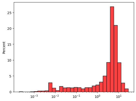
sns.histplot(
    x=dh_tom.data(
        "Zn_pct", 
        region="Zn_pct.notna()"
    ), 
    bins=30, 
    log_scale=True,
    stat='percent', 
    color='red'
)

<Axes: ylabel='Percent'>

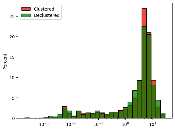
Using fairly the size of the drill spacing along x and y and using a large scale in z, we can compute the declustering weights.

declus_weight_mw = geo.moving_window_declus(
    obj=dh_tom, 
    obj_region="Zn_pct.notna()", 
    obj_attribute="Zn_pct", 
    diam_x=200, 
    diam_y=200, 
    diam_z=1500, 
    geometry="BALL"
)

print("Weight mean: ", declus_weight_mw.mean())

Weight mean:  1.0

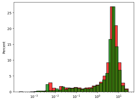
moving_window_declus outputs a numpy array of values with a mean of 1. The declustered histogram can also be visualised using seaborn and the weights parameter.

declus_weight_mw

array([0.77649391, 0.79988228, 0.8014917 , ..., 0.54269942, 0.54269942,
       0.5412247 ])

dh_tom["declus_weight_cd"] = "nan"
dh_tom.update_property("declus_weight_cd", data=declus_weight_mw, region="Zn_pct.notna()")

fig, ax = plt.subplots()
sns.histplot(
    x=dh_tom.data("Zn_pct", region="Zn_pct.notna()"), 
    bins=30, 
    log_scale=True, 
    stat='percent', 
    ax=ax, 
    color='red',
    label='Clustered'
)
sns.histplot(
    x=dh_tom.data("Zn_pct", region="Zn_pct.notna()"), 
    weights=declus_weight_mw, 
    bins=30, 
    log_scale=True, 
    stat='percent', 
    ax=ax, 
    color='green',
    label='Declustered'
)
ax.legend()
plt.show()

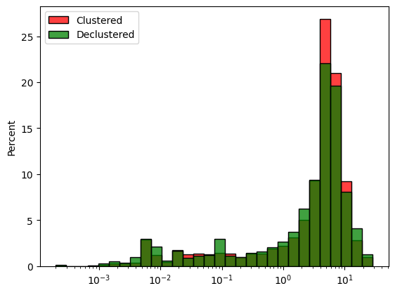
Cell Declustering is also available and works in the same manner.

declus_weight_cd = geo.cell_declustering(
    obj=dh_tom, 
    obj_region="Zn_pct.notna()", 
    obj_attribute="Zn_pct", 
    size_x=200, 
    size_y=200, 
    size_z=1500, 
    nb_off=50
)

print("Weights mean: ", declus_weight_cd.mean())

Weights mean:  1.0

fig, ax = plt.subplots()
sns.histplot(
    x=dh_tom.data("Zn_pct", region="Zn_pct.notna()"), 
    bins=30, 
    log_scale=True, 
    stat='percent', 
    ax=ax, 
    color='red',
    label='Clustered'
)
sns.histplot(
    x=dh_tom.data("Zn_pct", region="Zn_pct.notna()"), 
    weights=declus_weight_cd, 
    bins=30, 
    log_scale=True, 
    stat='percent', 
    ax=ax, 
    color='green',
    label='Declustered'
)
ax.legend()
plt.show()

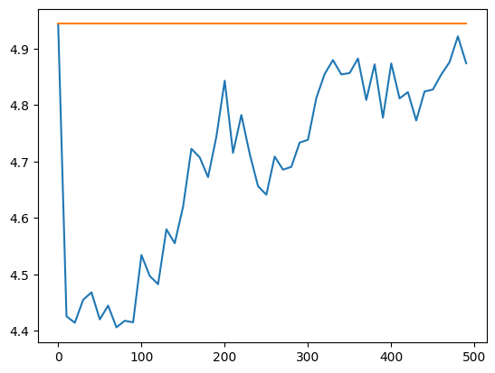
Declustering size of cell or ellipsoid can be found using a loop over different size and taking the size minimizing the mean of the data.

x_cs_cd = np.arange(0, 500, 10)
naive_mean = dh_tom.data("Zn_pct", "Zn_pct.notna()").mean()
var_mean_cd = [naive_mean]

for s in x_cs_cd[1:]:
    declus_weight_cd = geo.cell_declustering(
        obj=dh_tom, 
        obj_region="Zn_pct.notna()", 
        obj_attribute="Zn_pct", 
        size_x=s, 
        size_y=s, 
        size_z=1500, 
        nb_off=25
    )
    var_mean_cd.append(np.mean(declus_weight_cd * dh_tom.data("Zn_pct", "Zn_pct.notna()")))

fig, ax = plt.subplots()
ax.plot(
    x_cs_cd, 
    var_mean_cd,
    label="Declustered Mean"
)

ax.plot(
    x_cs_cd, 
    np.full((len(x_cs_cd)), naive_mean),
    label="Naive Mean"
)
plt.show()

Compositing

To perform compositing, we can create a new property called sample_length and analyse its distribution to find the most common lenght of the samples.

dh_tom.set_property(name="sample_length", data="TO - FROM")

dh_tom.user_properties()

['X_COLLAR',
 'Y_COLLAR',
 'Z_COLLAR',
 'X_M',
 'Y_M',
 'Z_M',
 'X_B',
 'Y_B',
 'Z_B',
 'X_E',
 'Y_E',
 'Z_E',
 'Ag_ppm',
 'Pb_pct',
 'Zn_pct',
 'BD_tonnes_m3',
 'Method',
 'Comment',
 'LowRecovery___85pct',
 'HoleType',
 'Year',
 'Property',
 'Prospect',
 'Grid',
 'NewsRelease',
 'Length_m',
 'declus_weight_cd',
 'sample_length']

dh_tom.describe(properties=['sample_length'])

	sample_length
count	2668.000000
mean	1.070956
std	0.417748
min	0.100000
25%	0.920000
50%	1.000000
75%	1.500000
max	4.600000

geo.histogram_plot(
    data=[{"object": dh_tom, "property": "sample_length"}], 
    width=650, 
    height=400,
    histnorm='percent',
    title=f'Sample length {len(dh_tom["sample_length"])}'
)

1m seems to be the most common value and will be used for compositing. Additional check such a histogram comparison can be made to asses the composite length.

dh_tom_2 = geo.compositing(
    drillholes=dh_tom,
    attribute_list=["Zn_pct", "Pb_pct", "Ag_ppm", "declus_weight_cd"],
    composit_len=1.,
    minimum_composit_len=0.3,
    residual_len=0.5,
    survey_df=survey_tom
)

2025-10-03 14:58:14,693 [INFO] GeoLime Project - |GEOLIME|.drillholes_compositing.py : Following survey mapping has been identified: {
    "AZIMUTH": "Azimuth",
    "DEPTH_SURVEY": "Depth_m",
    "DIP": "Dip",
    "HOLEID": "HoleID"
}

fig, ax = plt.subplots()
sns.histplot(
    x=dh_tom.data("Zn_pct", region="Zn_pct.notna()"), 
    bins=30, 
    log_scale=True, 
    stat='percent', 
    ax=ax, 
    color='red'
)
sns.histplot(x=dh_tom_2.data("Zn_pct", region="Zn_pct.notna()"), bins=30, log_scale=True, stat='percent', ax=ax, color='green')

<Axes: ylabel='Percent'>

DataFrame can also be created to have a summary comparing the original and composited Drillholes.

pd.DataFrame(
    [dh_tom.describe("Zn_pct"), dh_tom_2.describe("Zn_pct")], 
    index=['original', 'composited']
).T

	original	composited
count	2665.000000	2965.000000
mean	4.943900	4.901401
std	4.011429	3.752160
min	0.000200	0.000900
25%	1.800000	2.178125
50%	4.800000	4.824430
75%	6.700000	6.600000
max	28.600000	26.537500

Export to file for future use. geo files allow faster reading and writing.

dh_tom_2.to_file("../data/dh_tom_comp.geo")