Variography#
import geolime as geo
from pyproj import CRS
import numpy as np
import pyvista as pv
import json
pv.set_jupyter_backend('html')
geo.Project().set_crs(CRS("EPSG:20350"))
dh = geo.read_file("../data/domained_drillholes.geo")
dh.user_properties()
['X_COLLAR',
'Y_COLLAR',
'Z_COLLAR',
'X_M',
'Y_M',
'Z_M',
'X_B',
'Y_B',
'Z_B',
'X_E',
'Y_E',
'Z_E',
'Fe_pct',
'Al2O3',
'SiO2_pct',
'K2O_pct',
'CaO_pct',
'MgO_pct',
'TiO2_pct',
'P_pct',
'S_pct',
'Mn_pct',
'Fe_ox_ai',
'hem_over_goe',
'kaolin_abundance',
'kaolin_composition',
'wmAlsmai',
'wmAlsmci',
'carbai3pfit',
'carbci3pfit',
'Sample_ID',
'Fe',
'Fe2o3',
'P',
'S',
'SiO2',
'MnO',
'Mn',
'CaO',
'K2O',
'MgO',
'Na2O',
'TiO2',
'LOI_100',
'Depth',
'ellipsoidal_distance_1',
'ellipsoidal_distance_2',
'channel',
'domain_code',
'domain']
Experimental Variography and Variography Fitting is made in GeoLime using the following steps
Select the appropriate geostatistical domain in order to ensure stationnarity of the data
Experimental Variography in order to determine the direction of the anisotropy if there is one
Perform VarioMap/VarioContour in the XY Plan in order to determine the azimuth direction of continuity
Perfrom VarioMap/VarioContour in the Azimuth Plane in order to determine the dip of continuity
Perform VarioMap/VarioContour in the Dip Plane in order to determine the pitch of continuity
Once the anisotropy direction is found, compute the 1D experimental variograms needed for further automatic fitting.
Compute Downhole Variogram, which will be used to determine nugget effect.
Compute 1D Variogram in major direction
Compute 1D Variogram in semi-major direction
Compute 1D Variogram in minor direction
Perform Automatic Fitting of the variogram Model in a two step fashion
Automatic Fit of the Nugget Effect using the Downhole Variogram
Create an Empty Model consisting of the number and types of wanted structures
Automatic Fit of the Complete Model using the provided nugget value and set of constraints
Data Selection#
Subdividing Data into Domains: Dividing the deposit into domains or geologically homogeneous zones is crucial for accurate variography. Each domain should represent a population with consistent statistical properties. Performing variography on mixed populations without domaining can lead to misleading variograms that obscure the true spatial relationships.
Geological Domains have been made in Chapter 3 about geology modelling.
Geostatistical Dommains are here extracted from existing DXF file consisting of closed surfaces. For this study only the high grade domain of the channel is used and and modelled. In general and when possible, geostatistical domains are subparts of geological domains ensuring geology continuity but also stationnarity.
domain_solid = geo.datasets.load("rocklea_dome/domain_mesh.dxf")
domain_solid.name
'OreZone'
Here the domain_solid name is unclear and needs to be change. We will call it “channel_hg”, which referes to the domain of high grades values in the channel.
domain_solid.name = "channel_hg"
Solid object have the contains method allowing to check for any GeoLime object if their points lie inside the Solid. This create a new region on the interrogated object. The new region name is made of the following pattern : “in_{solid.name}”. In this case the new region name will be “in_channel_hg”.
domain_solid.contains(dh)
The flag of each composite of the Drillholes can be visualised in 3D.
domain_solid_pv = domain_solid.to_pyvista()
dh_pv = dh.to_pyvista('in_channel_hg')
plotter = pv.Plotter()
plotter.add_mesh(domain_solid_pv, style="wireframe")
plotter.add_mesh(dh_pv.tube(radius=20))
plotter.set_scale(zscale=10)
plotter.show()
As mentionned above the channel geological domains selects composites having similar lithology but does not guarantee stationnarity (meaning a single statistical population). Let’s see with an histogram if the geostatistical domain is accurate.
geo.histogram_plot(data=[{"object":dh, "property":"Fe_pct", "region":"in_channel_hg"}])
For simplicity and avoid any warning as we have “nan” data in the property of the study, we create a region “channel_hg” consisting of the points inside the solid, which have a measure of iron percentage. GeoLime does not silently ignore “nan” by default as they may represent an indication for non-standardised data or potential issues.
dh.set_region_condition("channel_hg", "in_channel_hg & Fe_pct.notna()")
VarioMap#
Determine Azimuth Direction#
Lags and tolerance value for experimental variography can be provided as List or numpy array of bin centers and bin semi width. For simplicity GeoLime provides 2 functions for te creation of lags:
generate_lags, which specify what is the lag distance, what is the lag tolerance, meaning if two consecutive bin are close to each other or if there is gap and the number of expected lag. This functions generates lag with the same bin size. Theplagparameter is recommended to be set to 50.
lags, tol = geo.generate_lags(lag=200, plag=50, nlags=15)
generate_lags_from_intervaltakes into input a list of list or a 2D numpy array consisting of the beggining and end of each lag. This requires manual definition of each lag but allows the user to have lags of different bin sizes.
geo.generate_lags_from_interval([[0, 50], [50, 100], [100, 200]])
lags, tol = geo.generate_lags(lag=200, plag=50, nlags=15)
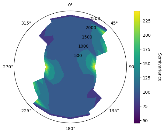
GeoLime provides experimental VarioMap and VarioContour in order to determine anisotropy direction. VarioMap allows to access to the actual semivariance of each lag in each direction, whereas VarioContour provides a more contrasted graphic, allowing easier trend identification. Both function takes into input a GeoLime object, the property of interest of the specifc object and a region, which can be None. They also take the defined lags and tolerance, a number of azimuth being the number of computed direction, and the angular tolerance in each direction.
geo.vario_map(
geo_object=dh,
attribute="Fe_pct",
region="channel_hg",
lags=lags,
tol=tol,
n_az=15,
atol=35
)
geo.vario_contour(
geo_object=dh,
attribute="Fe_pct",
region="channel_hg",
lags=lags,
tol=tol,
n_az=15,
atol=35
)
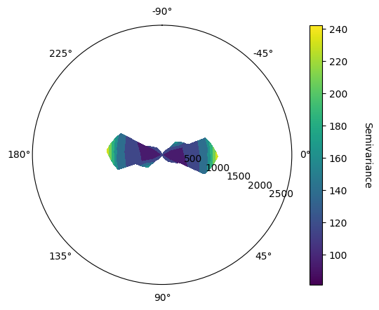
Determine Dip Direction#
In order to determine the dip direction, the function vario_contour_dip takes into input a given azimuth direction, here set to 0 as the variomap suggest a higher continuity in N00.
geo.vario_contour_dip(
geo_object=dh,
attribute="Fe_pct",
region="channel_hg",
lags=lags,
tol=tol,
azimuth=0,
n_dip=15,
atol=35
)
Determine Pitch Direction#
In order to determine the pitch direction, the function vario_contour_pitch takes into input a given azimuth direction, here set to 0 as the variomap suggest a higher continuity in N00 and a given dip, here set also to 0 as the vario_contour_dip suggest a higher continuity in the horizontal plane.
geo.vario_contour_pitch(
geo_object=dh,
attribute="Fe_pct",
region="channel_hg",
lags=lags,
tol=tol,
azimuth=0,
dip=0,
n_pitch=15,
atol=35
)
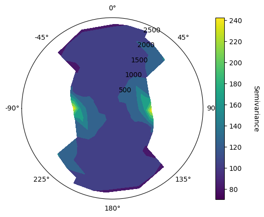
VarioMaps sugget major and minor preferential directions are N00 and N90, with dip and pitch values being null, indicating an anisotropy according to the stratigraphic plane.
major_azimuth = 0.
major_dip = 0.
major_pitch = 0.
Fitting a Covariance Model#
Model the Nugget Effect#
Automatic Fit of the Nugget Effect using the Downhole Variogram:
The nugget effect represents the small-scale variability or noise in the data, often attributed to measurement errors or variations below the sampling scale.
Downhole variograms are calculated using data pairs from within the same drill hole. Since these data pairs are closely spaced, they are particularly sensitive to short-scale variations, making them ideal for estimating the nugget effect.
Procedure:
Calculate the downhole variogram.
The nugget effect can often be visually estimated from the downhole variogram by observing the intercept of the variogram with the Y-axis (at a distance of zero).
Automated methods might involve fitting a simple model, like a spherical model with a very short range, to the first few lags of the downhole variogram. The nugget effect is then determined from the sill of this fitted model.
Experimental Downhole Variogram#
Here we create 10 lags of 1 meter, corresponding to the composite size.
lags_bh, tol_bh = geo.generate_lags(lag=1., plag=50, nlags=10.)
The variogram_downhole is useful for nugget determination.
vario_exp_bh = geo.variogram_downhole(
object=dh,
attribute="Fe_pct",
region="channel_hg",
lags=lags_bh,
tol=tol_bh
)
1D variograms can be displayed using the plot_semivariogram function. The number of pairs for each lag can be displayed on hover of each points.
geo.plot_semivariogram(
variograms=[vario_exp_bh],
display_npairs=True
)
1D Experimental variograms are pandas DataFrame.
vario_exp_bh
| lag | npairs | avgdist | vario | |
|---|---|---|---|---|
| 0 | 1.0 | 1601.0 | 1.0 | 38.453467 |
| 1 | 2.0 | 1530.0 | 2.0 | 60.226471 |
| 2 | 3.0 | 1460.0 | 3.0 | 71.746233 |
| 3 | 4.0 | 1394.0 | 4.0 | 80.208393 |
| 4 | 5.0 | 1324.0 | 5.0 | 83.884819 |
| 5 | 6.0 | 1256.0 | 6.0 | 83.457803 |
| 6 | 7.0 | 1192.0 | 7.0 | 84.465604 |
| 7 | 8.0 | 1124.0 | 8.0 | 82.919039 |
| 8 | 9.0 | 1057.0 | 9.0 | 83.146168 |
Automatic Fitting#
Create an Empty Model Consisting of the Number and Types of Wanted Structures:
Nested Structures: Variogram models often consist of multiple nested structures that represent different scales of spatial variation. Each structure is defined by its type (e.g., spherical, exponential, Gaussian) and its parameters (sill, range, anisotropy).
Selecting Structures: Deciding on the number and types of structures requires careful consideration of the experimental variograms and geological interpretation.
Example: If the experimental variograms suggest two distinct scales of variation, a nested model with two structures might be appropriate. The types of structures would be selected based on their shapes and how well they represent the observed behavior of the experimental variograms.
Empty Model: This step involves creating a placeholder variogram model with the chosen number and types of structures, but without specifying their parameters. The parameters will be determined in the next step.
nugget_model = geo.Nugget() + geo.Spherical()
geo.model_fit(
variograms=[vario_exp_bh],
cov=nugget_model
)
1D Experimental Variograms can be displayed with a model on the same figure using the model parameter. The model_angles parameter allows the plotting of multiple directions.
geo.plot_semivariogram(
variograms=[vario_exp_bh],
model=nugget_model,
model_angles=[{"azi":0, "dip":90, "pitch":90}],
display_npairs=True
)
print(nugget_model)
Model with 2 components
Component 1 :
Sill : 16.180169347228638
Covariance type : Nugget
Component 2 :
Sill : 65.82458159012036
Covariance type : Spherical
Scales : (8.978962628816342, 1.8513095968477695, 4.402431663209452)
Angles : (342.20485033812713, 8.323596504712468, -37.89222400913888)
Total sill = 82.004750937349
nugget_value = nugget_model.cov_elem_list[0].sill
Model the Sphericals#
Experimental Variograms along the XY plane#
Experimental variograms are then computed on the main direction, the main direction with a pitch of +/- 90 degrees being the semi-major axis, and the main direction with a dip of +/- 90 degrees being the minor direction.
Here scales of major and semi-major are of the same order of magnitude so we use the same lag definitions. A new set of lags will be used for the minor direction.
lags, tol = geo.generate_lags(lag=50, plag=50, nlags=10)
vario_exp_major = geo.variogram(
object=dh,
attribute="Fe_pct",
region="channel_hg",
geographic_azimuth=major_azimuth,
dip=major_dip,
pitch=major_pitch,
lags=lags,
tol=tol,
atol=40
)
vario_exp_semi_major = geo.variogram(
object=dh,
attribute="Fe_pct",
region="channel_hg",
geographic_azimuth=major_azimuth,
dip=major_dip,
pitch=major_pitch + 90,
lags=lags,
tol=tol,
atol=30
)
lags, tol = geo.generate_lags(lag=1., plag=50, nlags=10.)
vario_exp_minor = geo.variogram(
object=dh,
attribute="Fe_pct",
region="channel_hg",
geographic_azimuth=major_azimuth,
dip=major_dip + 90,
pitch=major_pitch + 90,
lags=lags,
tol=tol,
atol=30
)
geo.plot_semivariogram(
variograms=[vario_exp_major, vario_exp_semi_major, vario_exp_minor],
display_npairs=True
)
Experimental variogrphy here suggest the sill is already reached in the major and semi-major direction. Semi-major direction also has no value for small lags as data spacing is more important in this direction.
Automatic Fitting#
Automatic Fit of the Complete Model Using the Provided Nugget Value and Set of Constraints:
Nugget Value: The nugget effect determined in the first step is fixed in the model.
Constraints: Additional constraints might be imposed based on geological knowledge or practical considerations.
Automated Fitting Algorithms: The automatic fit relies on the Least Squuare method. The aim of this method is to minimize the weighted sum of squared differences between the experimental variogram values and the values predicted by the model. Three types of weighting are available :
Classical weighting : The weights are based on the number of data pairs used to calculate each experimental variogram value.
Inverse Distance Weighting : The weights are based on the number of data pairs used to calculate each experimental variogram value divided by the average distance of the pairs. This gives more impact on small scale variography.
Square Inverse Distance Weighting : The weights are based on the number of data pairs used to calculate each experimental variogram value divided by the square of the average distance of the pairs. This gives even more impact on small scale variography.
Visual Validation: Even with automatic fitting, it is crucial to visually assess the final variogram model and ensure that it provides a reasonable representation of the spatial variability observed in the experimental variograms.
For this study we decide to use a 2 structures model with a nugget effect.
model = geo.Nugget() + geo.Spherical() + geo.Spherical()
In this example as the sill is already reached it will be difficult to fit the 2 structures with only the experimental variograms. In order to force the algorithm to also model a second structure we specify the ratio of the remaining sill to give to each structure, ensuring both structures will have a non-neglectible value.
short_range_spherical_ratio = 0.6
long_range_spherical_ratio = 0.4
In the model_fit function, the constraints parameter allows to specify the defined sill ratios, but also to define the main direction of each structure. The experimental vaiography indicates that the sill is already reached for the existing value, so we set a maximum scale of 100m. We also do not see any anisotropy in the XY plane, so we set the scale for major and semi-major direction to be equal using the scale_expr constraint.
geo.model_fit(
variograms=[
vario_exp_major,
vario_exp_semi_major,
vario_exp_minor
],
cov=model,
constraints=[
{"sill_fixed":nugget_value},
{
"sill_max": short_range_spherical_ratio * (vario_exp_major.attrs["variable_var"] - nugget_value),
"angle_fixed_0": major_azimuth,
"angle_fixed_1": major_dip,
"angle_fixed_2": major_pitch,
"scale_max_0": 100,
"scale_expr_1": "scale_0_1"
},
{
"sill_max": long_range_spherical_ratio * (vario_exp_major.attrs["variable_var"] - nugget_value),
"angle_fixed_0": major_azimuth,
"angle_fixed_1": major_dip,
"angle_fixed_2": major_pitch,
"scale_max_0": 100,
"scale_expr_1": "scale_0_2"
}
]
)
geo.plot_semivariogram(
variograms=[
vario_exp_major,
vario_exp_semi_major,
vario_exp_minor
],
model=model,
model_angles=[
{"azi":major_azimuth, "dip":major_dip, "pitch":major_pitch},
{"azi":major_azimuth, "dip":major_dip, "pitch":major_pitch + 90},
{"azi":major_azimuth, "dip":major_dip + 90, "pitch":major_pitch + 90}
],
display_npairs=True,
variogram_colors=['green', 'blue', 'orange']
)
print(model)
Model with 3 components
Component 1 :
Sill : 16.180169347228638
Covariance type : Nugget
Component 2 :
Sill : 45.5685762475326
Covariance type : Spherical
Scales : (65.3257291940125, 65.3257291940125, 3.545335034976783)
Angles : (0.0, 0.0, 0.0)
Component 3 :
Sill : 30.335529862326037
Covariance type : Spherical
Scales : (81.56012140210935, 81.56012140210935, 11.075987065017534)
Angles : (0.0, 0.0, 0.0)
Total sill = 92.08427545708727
Write model to a file#
Covariance models can then be exported to different types of files for reuse. For example they can be stored into json file comparable to LeapFrog Variogram lfv files.
cov_dict = {}
cov_dict["nugget"] = model.cov_elem_list[0].sill
cov_dict["sill"] = model.sill - model.cov_elem_list[0].sill
cov_dict["data_variance"] = dh.data("Fe_pct", region="channel_hg").var()
cov_dict["structures"] = []
for i, c in enumerate(range(1, len(model.cov_elem_list))):
cov_dict["structures"].append({})
cov_dict["structures"][i]["contribution"] = model.cov_elem_list[c].sill
cov_dict["structures"][i]["anisotropy"] = {}
cov_dict["structures"][i]["anisotropy"]["ranges"] = {}
cov_dict["structures"][i]["anisotropy"]["ranges"]["major"] = model.cov_elem_list[c].metric.scales[0]
cov_dict["structures"][i]["anisotropy"]["ranges"]["semi-major"] = model.cov_elem_list[c].metric.scales[1]
cov_dict["structures"][i]["anisotropy"]["ranges"]["minor"] = model.cov_elem_list[c].metric.scales[2]
cov_dict["structures"][i]["anisotropy"]["rotation"] = {}
cov_dict["structures"][i]["anisotropy"]["rotation"]["dip_direction"] = model.cov_elem_list[c].metric.angles[0]
cov_dict["structures"][i]["anisotropy"]["rotation"]["dip"] = model.cov_elem_list[c].metric.angles[1]
cov_dict["structures"][i]["anisotropy"]["rotation"]["pitch"] = model.cov_elem_list[c].metric.angles[2]
cov_dict["structures"][i]["structure_type"] = model.cov_elem_list[c].type
with open('../data/cov_model.json', 'w') as fp:
json.dump(cov_dict, fp)