Comparison of the assay and hyperspectral datas#
The assay file contains the Hole_ID of every drillhole, their position in the hole, the chemical composition of the sample (Fe, Fe2O3, P, S, SiO2, Al2O3, MnO, Mn, CaO, K2O, MgO, Na2O, TiO2) and the loss-on-ignition percentage.
The hyperspectral file contains the Hole_ID of every drillhole, their position in the hole, the chemical composition of each sample (Fe, Al2O3, SiO2, K2O, CaO, MgO, TiO2, P, S, Mn), the loss-on-ignition percentage and other informations about the minerals in the sample.
The common data between these two files are the Hole_ID, the depth, most columns about chemical composition (Fe, Al2O3, SiO2, K2O, CaO, MgO, TiO2, P, S, Mn) and the loss-on-ignition percentage.
The aim of this notebook is to compare the two files in order to find the common holes and compare the values in identical holes in order to assess lab results from the two different techniques beign hyperspectral and XRF.
import numpy as np
import pandas as pd
import geolime as geo
import seaborn as sns
Format Pandas display for clarity and readability
pd.set_option("display.max_rows", 10)
pd.set_option("display.max_columns", 500)
We want to compare the Hole_ID of the assay and hyperspectral file to know if they have some drillholes in common.
First we need to import these data from .csv files.
Merging Interval Files#
Assay File reading and formatting#
assay = geo.datasets.load("rocklea_dome/assay.csv")
assay
| Hole_ID | From | To | Sample_ID | Fe | Fe2o3 | P | S | SiO2 | Al2O3 | MnO | Mn | CaO | K2O | MgO | Na2O | TiO2 | LOI | LOI_100 | |
|---|---|---|---|---|---|---|---|---|---|---|---|---|---|---|---|---|---|---|---|
| 0 | RKC001 | 35.0 | 36.0 | 36.0 | 0.0 | 0 | 0 | 0 | 0.0 | 0.0 | 0.0 | 0.0 | 0.0 | 0.0 | 0.0 | 0.0 | 0 | 0 | 0.0 |
| 1 | RKC001 | 36.0 | 37.0 | 37.0 | 0.0 | 0 | 0 | 0 | 0.0 | 0.0 | 0.0 | 0.0 | 0.0 | 0.0 | 0.0 | 0.0 | 0 | 0 | 0.0 |
| 2 | RKC001 | 37.0 | 38.0 | 38.0 | 0.0 | 0 | 0 | 0 | 0.0 | 0.0 | 0.0 | 0.0 | 0.0 | 0.0 | 0.0 | 0.0 | 0 | 0 | 0.0 |
| 3 | RKC001 | 38.0 | 39.0 | 39.0 | 0.0 | 0 | 0 | 0 | 0.0 | 0.0 | 0.0 | 0.0 | 0.0 | 0.0 | 0.0 | 0.0 | 0 | 0 | 0.0 |
| 4 | RKC001 | 39.0 | 40.0 | 40.0 | 0.0 | 0 | 0 | 0 | 0.0 | 0.0 | 0.0 | 0.0 | 0.0 | 0.0 | 0.0 | 0.0 | 0 | 0 | 0.0 |
| ... | ... | ... | ... | ... | ... | ... | ... | ... | ... | ... | ... | ... | ... | ... | ... | ... | ... | ... | ... |
| 17461 | RKD010 | 0.0 | 44.0 | NaN | 0.0 | 0 | 0 | 0 | 0.0 | 0.0 | 0.0 | 0.0 | 0.0 | 0.0 | 0.0 | 0.0 | 0 | 0 | 0.0 |
| 17462 | RKD011 | 0.0 | 42.5 | NaN | 0.0 | 0 | 0 | 0 | 0.0 | 0.0 | 0.0 | 0.0 | 0.0 | 0.0 | 0.0 | 0.0 | 0 | 0 | 0.0 |
| 17463 | RKD013 | 0.0 | 30.0 | NaN | 0.0 | 0 | 0 | 0 | 0.0 | 0.0 | 0.0 | 0.0 | 0.0 | 0.0 | 0.0 | 0.0 | 0 | 0 | 0.0 |
| 17464 | RKD014 | 0.0 | 44.0 | NaN | 0.0 | 0 | 0 | 0 | 0.0 | 0.0 | 0.0 | 0.0 | 0.0 | 0.0 | 0.0 | 0.0 | 0 | 0 | 0.0 |
| 17465 | RKD015 | 0.0 | 41.0 | NaN | 0.0 | 0 | 0 | 0 | 0.0 | 0.0 | 0.0 | 0.0 | 0.0 | 0.0 | 0.0 | 0.0 | 0 | 0 | 0.0 |
17466 rows × 19 columns
Some columns have string values named LNR, replacing them to NaN will allow comparisons with other number columns. Using the .dtypes information allows to find out wich columns are considered numerical (float64 or int64) and which column are considered as string/text and are identified by Pandas as object.
assay.dtypes
Hole_ID       object
From         float64
To           float64
Sample_ID    float64
Fe           float64
              ...
MgO          float64
Na2O         float64
TiO2          object
LOI           object
LOI_100      float64
Length: 19, dtype: object
Using the eq method makes it easy to find if any column has a value equals to “LNR”.
assay.eq("LNR").any()
Hole_ID      False
From         False
To           False
Sample_ID    False
Fe           False
             ...
MgO          False
Na2O         False
TiO2          True
LOI           True
LOI_100      False
Length: 19, dtype: bool
Replacing the problematic value by nan (which means ‘not a number’ but is considered as a numeric information by Pandas and Numpy) and then making sure the column are converted into numeric values is done in two step.
assay.replace("LNR", np.nan, inplace=True)
assay[["P", "S", "TiO2", "LOI"]] = assay[["P", "S", "TiO2", "LOI"]].apply(pd.to_numeric)
Hyperspec File reading#
hyperspec = pd.read_csv("../data/hyperspec.csv")
hyperspec
| Hole_ID | From | To | Fe_pct | Al2O3 | SiO2_pct | K2O_pct | CaO_pct | MgO_pct | TiO2_pct | P_pct | S_pct | Mn_pct | LOI | Fe_ox_ai | hem_over_goe | kaolin_abundance | kaolin_composition | wmAlsmai | wmAlsmci | carbai3pfit | carbci3pfit | |
|---|---|---|---|---|---|---|---|---|---|---|---|---|---|---|---|---|---|---|---|---|---|---|
| 0 | RKC278 | 0.0 | 1.0 | NaN | NaN | NaN | NaN | NaN | NaN | NaN | NaN | NaN | NaN | NaN | 0.1290 | 891.13 | 0.0374 | 0.999 | NaN | NaN | NaN | NaN |
| 1 | RKC278 | 1.0 | 2.0 | NaN | NaN | NaN | NaN | NaN | NaN | NaN | NaN | NaN | NaN | NaN | 0.1460 | 892.68 | 0.0269 | 1.006 | NaN | NaN | NaN | NaN |
| 2 | RKC278 | 2.0 | 3.0 | NaN | NaN | NaN | NaN | NaN | NaN | NaN | NaN | NaN | NaN | NaN | 0.1650 | 895.24 | NaN | NaN | NaN | NaN | NaN | NaN |
| 3 | RKC278 | 3.0 | 4.0 | NaN | NaN | NaN | NaN | NaN | NaN | NaN | NaN | NaN | NaN | NaN | 0.1000 | 893.34 | NaN | NaN | 0.0545 | 2211.83 | NaN | NaN |
| 4 | RKC278 | 4.0 | 5.0 | NaN | NaN | NaN | NaN | NaN | NaN | NaN | NaN | NaN | NaN | NaN | 0.0445 | 910.32 | NaN | NaN | NaN | NaN | 0.111 | 2312.89 |
| ... | ... | ... | ... | ... | ... | ... | ... | ... | ... | ... | ... | ... | ... | ... | ... | ... | ... | ... | ... | ... | ... | ... |
| 7103 | RKC485 | 41.0 | 42.0 | 28.0 | 9.80 | 39.05 | 0.037 | 0.08 | 0.22 | 1.078 | 0.027 | 0.006 | 0.12 | 9.00 | 0.2210 | 912.17 | 0.0322 | 1.004 | NaN | NaN | NaN | NaN |
| 7104 | RKC485 | 42.0 | 43.0 | 39.0 | 7.67 | 25.15 | 0.029 | 0.09 | 0.25 | 0.689 | 0.046 | 0.008 | 0.11 | 10.11 | 0.1200 | 912.43 | 0.1140 | 1.027 | NaN | NaN | NaN | NaN |
| 7105 | RKC485 | 43.0 | 44.0 | 16.0 | 20.23 | 43.41 | 0.177 | 0.17 | 0.34 | 1.617 | 0.020 | 0.018 | 0.05 | 10.80 | 0.0956 | 888.81 | 0.0306 | 1.012 | NaN | NaN | NaN | NaN |
| 7106 | RKC485 | 44.0 | 45.0 | 12.0 | 12.53 | 50.24 | 0.060 | 0.26 | 0.25 | 1.473 | 0.006 | 0.779 | 0.03 | 16.18 | 0.0378 | 958.21 | 0.1100 | 1.025 | NaN | NaN | NaN | NaN |
| 7107 | RKD015 | 0.0 | 1.0 | NaN | NaN | NaN | NaN | NaN | NaN | NaN | NaN | NaN | NaN | NaN | NaN | NaN | NaN | NaN | NaN | NaN | NaN | NaN |
7108 rows × 22 columns
Merge Preparation#
The comparison of the two datasets require to have the list of the different Hole_ID of both files. These lists also need to be turned into sets in order to compare them.
The set type ensures there are no duplicate values, being useful here as Hole_ID are unique identifier.
colonne_assay = set(assay["Hole_ID"])
colonne_hyperspec = set(hyperspec["Hole_ID"])
Now we have two sets with the different drill core that have been analyzed for each method.
The length of each set indicates how many holes are present in each dataset.
len(colonne_assay)
500
len(colonne_hyperspec)
192
The two file do not have the same amount of hole. The set type enables ensemble query such as intersection/union/difference. The intersection here will allow to find the common hole between the two dataset.
Next command will search all the Hole_ID both in the assay and hyperspec file.
intersection = colonne_assay.intersection(colonne_hyperspec)
len(intersection)
192
The intersection of these two files has the same length as the smallest set, so every Hole_ID of the hyperspectral file are in the assay.
The drill cores of the hyperspectral file are included in the assay file. Now we want to see if the common columns between these two files have the same values. First we need to filter the DataFrame of the assay file in order to keep only the Hole_ID that are in common with the hyperspectral file.
intersection = list(intersection)
filtred_assay = assay[assay["Hole_ID"].isin(intersection)]
filtred_assay
| Hole_ID | From | To | Sample_ID | Fe | Fe2o3 | P | S | SiO2 | Al2O3 | MnO | Mn | CaO | K2O | MgO | Na2O | TiO2 | LOI | LOI_100 | |
|---|---|---|---|---|---|---|---|---|---|---|---|---|---|---|---|---|---|---|---|
| 9778 | RKC278 | 0.0 | 1.0 | 10001.0 | 0.00 | 0 | 0.000 | 0.000 | 0.00 | 0.00 | 0.0 | 0.000 | 0.00 | 0.000 | 0.00 | 0.0 | 0.000 | 0.00 | 0.0 |
| 9779 | RKC278 | 1.0 | 2.0 | 10002.0 | 0.00 | 0 | 0.000 | 0.000 | 0.00 | 0.00 | 0.0 | 0.000 | 0.00 | 0.000 | 0.00 | 0.0 | 0.000 | 0.00 | 0.0 |
| 9780 | RKC278 | 2.0 | 3.0 | 10003.0 | 0.00 | 0 | 0.000 | 0.000 | 0.00 | 0.00 | 0.0 | 0.000 | 0.00 | 0.000 | 0.00 | 0.0 | 0.000 | 0.00 | 0.0 |
| 9781 | RKC278 | 3.0 | 4.0 | 10004.0 | 0.00 | 0 | 0.000 | 0.000 | 0.00 | 0.00 | 0.0 | 0.000 | 0.00 | 0.000 | 0.00 | 0.0 | 0.000 | 0.00 | 0.0 |
| 9782 | RKC278 | 4.0 | 5.0 | 10005.0 | 0.00 | 0 | 0.000 | 0.000 | 0.00 | 0.00 | 0.0 | 0.000 | 0.00 | 0.000 | 0.00 | 0.0 | 0.000 | 0.00 | 0.0 |
| ... | ... | ... | ... | ... | ... | ... | ... | ... | ... | ... | ... | ... | ... | ... | ... | ... | ... | ... | ... |
| 17379 | RKC485 | 13.0 | 14.0 | 17215.0 | 10.73 | 0 | 0.003 | 0.021 | 48.30 | 21.94 | 0.0 | 0.001 | 0.92 | 0.055 | 2.04 | 0.0 | 1.379 | 9.84 | 0.0 |
| 17380 | RKC485 | 10.0 | 11.0 | 17212.0 | 11.74 | 0 | 0.005 | 0.023 | 46.01 | 19.45 | 0.0 | 0.001 | 2.23 | 0.063 | 2.39 | 0.0 | 1.699 | 10.59 | 0.0 |
| 17381 | RKC485 | 11.0 | 12.0 | 17213.0 | 11.25 | 0 | 0.002 | 0.010 | 48.25 | 18.76 | 0.0 | 0.001 | 1.84 | 0.054 | 2.49 | 0.0 | 1.407 | 9.92 | 0.0 |
| 17382 | RKC485 | 12.0 | 13.0 | 17214.0 | 8.41 | 0 | 0.001 | 0.007 | 49.28 | 19.61 | 0.0 | 0.001 | 3.75 | 0.058 | 2.58 | 0.0 | 1.239 | 11.19 | 0.0 |
| 17465 | RKD015 | 0.0 | 41.0 | NaN | 0.00 | 0 | 0.000 | 0.000 | 0.00 | 0.00 | 0.0 | 0.000 | 0.00 | 0.000 | 0.00 | 0.0 | 0.000 | 0.00 | 0.0 |
7235 rows × 19 columns
The next operation will delete every sample of the assay file that is not in the hyperspectral file and make sure that we have the exact same number of Hole_ID in both files.
assay_final = hyperspec.merge(filtred_assay, on=["Hole_ID", "From", "To"], how="left")
assay_final.sort_values(by=["Hole_ID", "From"], inplace=True)
assay_final
| Hole_ID | From | To | Fe_pct | Al2O3_x | SiO2_pct | K2O_pct | CaO_pct | MgO_pct | TiO2_pct | P_pct | S_pct | Mn_pct | LOI_x | Fe_ox_ai | hem_over_goe | kaolin_abundance | kaolin_composition | wmAlsmai | wmAlsmci | carbai3pfit | carbci3pfit | Sample_ID | Fe | Fe2o3 | P | S | SiO2 | Al2O3_y | MnO | Mn | CaO | K2O | MgO | Na2O | TiO2 | LOI_y | LOI_100 | |
|---|---|---|---|---|---|---|---|---|---|---|---|---|---|---|---|---|---|---|---|---|---|---|---|---|---|---|---|---|---|---|---|---|---|---|---|---|---|---|
| 0 | RKC278 | 0.0 | 1.0 | NaN | NaN | NaN | NaN | NaN | NaN | NaN | NaN | NaN | NaN | NaN | 0.1290 | 891.13 | 0.0374 | 0.999 | NaN | NaN | NaN | NaN | 10001.0 | 0.00 | 0.0 | 0.000 | 0.000 | 0.00 | 0.00 | 0.0 | 0.00 | 0.00 | 0.000 | 0.00 | 0.0 | 0.000 | 0.00 | 0.0 |
| 1 | RKC278 | 1.0 | 2.0 | NaN | NaN | NaN | NaN | NaN | NaN | NaN | NaN | NaN | NaN | NaN | 0.1460 | 892.68 | 0.0269 | 1.006 | NaN | NaN | NaN | NaN | 10002.0 | 0.00 | 0.0 | 0.000 | 0.000 | 0.00 | 0.00 | 0.0 | 0.00 | 0.00 | 0.000 | 0.00 | 0.0 | 0.000 | 0.00 | 0.0 |
| 2 | RKC278 | 2.0 | 3.0 | NaN | NaN | NaN | NaN | NaN | NaN | NaN | NaN | NaN | NaN | NaN | 0.1650 | 895.24 | NaN | NaN | NaN | NaN | NaN | NaN | 10003.0 | 0.00 | 0.0 | 0.000 | 0.000 | 0.00 | 0.00 | 0.0 | 0.00 | 0.00 | 0.000 | 0.00 | 0.0 | 0.000 | 0.00 | 0.0 |
| 3 | RKC278 | 3.0 | 4.0 | NaN | NaN | NaN | NaN | NaN | NaN | NaN | NaN | NaN | NaN | NaN | 0.1000 | 893.34 | NaN | NaN | 0.0545 | 2211.83 | NaN | NaN | 10004.0 | 0.00 | 0.0 | 0.000 | 0.000 | 0.00 | 0.00 | 0.0 | 0.00 | 0.00 | 0.000 | 0.00 | 0.0 | 0.000 | 0.00 | 0.0 |
| 4 | RKC278 | 4.0 | 5.0 | NaN | NaN | NaN | NaN | NaN | NaN | NaN | NaN | NaN | NaN | NaN | 0.0445 | 910.32 | NaN | NaN | NaN | NaN | 0.111 | 2312.89 | 10005.0 | 0.00 | 0.0 | 0.000 | 0.000 | 0.00 | 0.00 | 0.0 | 0.00 | 0.00 | 0.000 | 0.00 | 0.0 | 0.000 | 0.00 | 0.0 |
| ... | ... | ... | ... | ... | ... | ... | ... | ... | ... | ... | ... | ... | ... | ... | ... | ... | ... | ... | ... | ... | ... | ... | ... | ... | ... | ... | ... | ... | ... | ... | ... | ... | ... | ... | ... | ... | ... | ... |
| 7103 | RKC485 | 41.0 | 42.0 | 28.0 | 9.80 | 39.05 | 0.037 | 0.08 | 0.22 | 1.078 | 0.027 | 0.006 | 0.12 | 9.00 | 0.2210 | 912.17 | 0.0322 | 1.004 | NaN | NaN | NaN | NaN | 17244.0 | 28.01 | 0.0 | 0.027 | 0.006 | 39.05 | 9.80 | 0.0 | 0.12 | 0.08 | 0.037 | 0.22 | 0.0 | 1.078 | 9.00 | 0.0 |
| 7104 | RKC485 | 42.0 | 43.0 | 39.0 | 7.67 | 25.15 | 0.029 | 0.09 | 0.25 | 0.689 | 0.046 | 0.008 | 0.11 | 10.11 | 0.1200 | 912.43 | 0.1140 | 1.027 | NaN | NaN | NaN | NaN | 17245.0 | 38.60 | 0.0 | 0.046 | 0.008 | 25.15 | 7.67 | 0.0 | 0.11 | 0.09 | 0.029 | 0.25 | 0.0 | 0.689 | 10.11 | 0.0 |
| 7105 | RKC485 | 43.0 | 44.0 | 16.0 | 20.23 | 43.41 | 0.177 | 0.17 | 0.34 | 1.617 | 0.020 | 0.018 | 0.05 | 10.80 | 0.0956 | 888.81 | 0.0306 | 1.012 | NaN | NaN | NaN | NaN | 17246.0 | 15.53 | 0.0 | 0.020 | 0.018 | 43.41 | 20.23 | 0.0 | 0.05 | 0.17 | 0.177 | 0.34 | 0.0 | 1.617 | 10.80 | 0.0 |
| 7106 | RKC485 | 44.0 | 45.0 | 12.0 | 12.53 | 50.24 | 0.060 | 0.26 | 0.25 | 1.473 | 0.006 | 0.779 | 0.03 | 16.18 | 0.0378 | 958.21 | 0.1100 | 1.025 | NaN | NaN | NaN | NaN | 17247.0 | 12.22 | 0.0 | 0.006 | 0.779 | 50.24 | 12.53 | 0.0 | 0.03 | 0.26 | 0.060 | 0.25 | 0.0 | 1.473 | 16.18 | 0.0 |
| 7107 | RKD015 | 0.0 | 1.0 | NaN | NaN | NaN | NaN | NaN | NaN | NaN | NaN | NaN | NaN | NaN | NaN | NaN | NaN | NaN | NaN | NaN | NaN | NaN | NaN | NaN | NaN | NaN | NaN | NaN | NaN | NaN | NaN | NaN | NaN | NaN | NaN | NaN | NaN | NaN |
7108 rows × 38 columns
Merged Data Verification#
This new file allows to make comparison between the data from the assay file (obtain by a XRF analysis) and the data from the hyperspectral analysis.
First we can compare the Fe weight percentage :
sns.scatterplot(data=assay_final, x="Fe", y="Fe_pct");
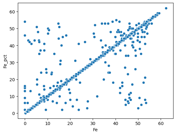
Most of the measures are similar for both methods. We can do the same for the Al2O3 weight percentage :
sns.scatterplot(data=assay_final, x="Al2O3_x", y="Al2O3_y");

assay_final.drop(columns=["Al2O3_y", "LOI_x", "LOI_y"], inplace=True)
assay_final.rename(columns={"Al2O3_x": "Al2O3"}, inplace=True)
assay_final.to_csv("../data/assay_hyper.csv", index=False)