Comparison of the hyperspectral and assay data#
Now that we have cleaned the hyperspectral data (hyperspec.csv) (See Section 0 - Data Cleaning), we can begin to compare the hyperspectral data with the geochemical assay data (assay.csv).
For every drillhole, the assay file contains the Hole_ID, depth, the chemical composition of the sample (Fe, Fe2O3, P, S, SiO2, Al2O3, MnO, Mn, CaO, K2O, MgO, Na2O, TiO2) and the loss-on-ignition percentage.
The hyperspec file contains the Hole_ID of every drillhole, depth, the chemical composition of each sample (Fe, Al2O3, SiO2, K2O, CaO, MgO, TiO2, P, S, Mn), the loss-on-ignition percentage and other information about the minerals in the sample.
The common data between these two files are the Hole_ID, the depth, the loss-on-ignition percentage, and most columns about chemical composition (Fe, Al2O3, SiO2, K2O, CaO, MgO, TiO2, P, S, Mn).
The aim of this notebook is to compare the two files in order to find the common holes and compare the values in identical holes in order to assess lab results from the two different techniques (hyperspectral and XRF).
import numpy as np
import pandas as pd
import geolime as geo
import seaborn as sns
Format Pandas display for clarity and readability
pd.set_option("display.max_rows", 20)
pd.set_option("display.max_columns", 500)
We want to compare the Hole_ID of the assay and hyperspectral file to know if they have some drillholes in common.
First we need to import these data from .csv files.
Merging Interval Files#
Assay File reading and formatting#
assay = geo.datasets.load("rocklea_dome/assay.csv")
assay
| Hole_ID | From | To | Sample_ID | Fe | Fe2o3 | P | S | SiO2 | Al2O3 | MnO | Mn | CaO | K2O | MgO | Na2O | TiO2 | LOI | LOI_100 | |
|---|---|---|---|---|---|---|---|---|---|---|---|---|---|---|---|---|---|---|---|
| 0 | RKC001 | 35.0 | 36.0 | 36.0 | 0.0 | 0 | 0 | 0 | 0.0 | 0.0 | 0.0 | 0.0 | 0.0 | 0.0 | 0.0 | 0.0 | 0 | 0 | 0.0 |
| 1 | RKC001 | 36.0 | 37.0 | 37.0 | 0.0 | 0 | 0 | 0 | 0.0 | 0.0 | 0.0 | 0.0 | 0.0 | 0.0 | 0.0 | 0.0 | 0 | 0 | 0.0 |
| 2 | RKC001 | 37.0 | 38.0 | 38.0 | 0.0 | 0 | 0 | 0 | 0.0 | 0.0 | 0.0 | 0.0 | 0.0 | 0.0 | 0.0 | 0.0 | 0 | 0 | 0.0 |
| 3 | RKC001 | 38.0 | 39.0 | 39.0 | 0.0 | 0 | 0 | 0 | 0.0 | 0.0 | 0.0 | 0.0 | 0.0 | 0.0 | 0.0 | 0.0 | 0 | 0 | 0.0 |
| 4 | RKC001 | 39.0 | 40.0 | 40.0 | 0.0 | 0 | 0 | 0 | 0.0 | 0.0 | 0.0 | 0.0 | 0.0 | 0.0 | 0.0 | 0.0 | 0 | 0 | 0.0 |
| ... | ... | ... | ... | ... | ... | ... | ... | ... | ... | ... | ... | ... | ... | ... | ... | ... | ... | ... | ... |
| 17461 | RKD010 | 0.0 | 44.0 | NaN | 0.0 | 0 | 0 | 0 | 0.0 | 0.0 | 0.0 | 0.0 | 0.0 | 0.0 | 0.0 | 0.0 | 0 | 0 | 0.0 |
| 17462 | RKD011 | 0.0 | 42.5 | NaN | 0.0 | 0 | 0 | 0 | 0.0 | 0.0 | 0.0 | 0.0 | 0.0 | 0.0 | 0.0 | 0.0 | 0 | 0 | 0.0 |
| 17463 | RKD013 | 0.0 | 30.0 | NaN | 0.0 | 0 | 0 | 0 | 0.0 | 0.0 | 0.0 | 0.0 | 0.0 | 0.0 | 0.0 | 0.0 | 0 | 0 | 0.0 |
| 17464 | RKD014 | 0.0 | 44.0 | NaN | 0.0 | 0 | 0 | 0 | 0.0 | 0.0 | 0.0 | 0.0 | 0.0 | 0.0 | 0.0 | 0.0 | 0 | 0 | 0.0 |
| 17465 | RKD015 | 0.0 | 41.0 | NaN | 0.0 | 0 | 0 | 0 | 0.0 | 0.0 | 0.0 | 0.0 | 0.0 | 0.0 | 0.0 | 0.0 | 0 | 0 | 0.0 |
17466 rows × 19 columns
Some columns have string values named LNR, replacing them with NaN values will allow comparisons with other numerical columns. Here the dtype function is used to discriminate columns with strings (object) against columns with numerical values only (float64, int64)
assay.dtypes
Hole_ID       object
From         float64
To           float64
Sample_ID    float64
Fe           float64
Fe2o3          int64
P             object
S             object
SiO2         float64
Al2O3        float64
MnO          float64
Mn           float64
CaO          float64
K2O          float64
MgO          float64
Na2O         float64
TiO2          object
LOI           object
LOI_100      float64
dtype: object
We can then determine which columns contain the value LNR using the eq function.
assay.eq("LNR").any()
Hole_ID      False
From         False
To           False
Sample_ID    False
Fe           False
Fe2o3        False
P             True
S             True
SiO2         False
Al2O3        False
MnO          False
Mn           False
CaO          False
K2O          False
MgO          False
Na2O         False
TiO2          True
LOI           True
LOI_100      False
dtype: bool
A replace function is then used to replace LNR values with NaN values.
All columns which previously held LNR values are then set to numeric dtypes using the .apply(pd.to_numeric) function.
assay.replace("LNR", np.nan, inplace=True)
assay[["P", "S", "TiO2", "LOI"]] = assay[["P", "S", "TiO2", "LOI"]].apply(pd.to_numeric)
Hyperspec File reading#
hyperspec = pd.read_csv("../data/hyperspec.csv")
hyperspec
| Hole_ID | From | To | Fe_pct | Al2O3 | SiO2_pct | K2O_pct | CaO_pct | MgO_pct | TiO2_pct | P_pct | S_pct | Mn_pct | LOI | Fe_ox_ai | hem_over_goe | kaolin_abundance | kaolin_composition | wmAlsmai | wmAlsmci | carbai3pfit | carbci3pfit | |
|---|---|---|---|---|---|---|---|---|---|---|---|---|---|---|---|---|---|---|---|---|---|---|
| 0 | RKC278 | 0.0 | 1.0 | NaN | NaN | NaN | NaN | NaN | NaN | NaN | NaN | NaN | NaN | NaN | 0.1290 | 891.13 | 0.0374 | 0.999 | NaN | NaN | NaN | NaN |
| 1 | RKC278 | 1.0 | 2.0 | NaN | NaN | NaN | NaN | NaN | NaN | NaN | NaN | NaN | NaN | NaN | 0.1460 | 892.68 | 0.0269 | 1.006 | NaN | NaN | NaN | NaN |
| 2 | RKC278 | 2.0 | 3.0 | NaN | NaN | NaN | NaN | NaN | NaN | NaN | NaN | NaN | NaN | NaN | 0.1650 | 895.24 | NaN | NaN | NaN | NaN | NaN | NaN |
| 3 | RKC278 | 3.0 | 4.0 | NaN | NaN | NaN | NaN | NaN | NaN | NaN | NaN | NaN | NaN | NaN | 0.1000 | 893.34 | NaN | NaN | 0.0545 | 2211.83 | NaN | NaN |
| 4 | RKC278 | 4.0 | 5.0 | NaN | NaN | NaN | NaN | NaN | NaN | NaN | NaN | NaN | NaN | NaN | 0.0445 | 910.32 | NaN | NaN | NaN | NaN | 0.111 | 2312.89 |
| ... | ... | ... | ... | ... | ... | ... | ... | ... | ... | ... | ... | ... | ... | ... | ... | ... | ... | ... | ... | ... | ... | ... |
| 7103 | RKC485 | 41.0 | 42.0 | 28.0 | 9.80 | 39.05 | 0.037 | 0.08 | 0.22 | 1.078 | 0.027 | 0.006 | 0.12 | 9.00 | 0.2210 | 912.17 | 0.0322 | 1.004 | NaN | NaN | NaN | NaN |
| 7104 | RKC485 | 42.0 | 43.0 | 39.0 | 7.67 | 25.15 | 0.029 | 0.09 | 0.25 | 0.689 | 0.046 | 0.008 | 0.11 | 10.11 | 0.1200 | 912.43 | 0.1140 | 1.027 | NaN | NaN | NaN | NaN |
| 7105 | RKC485 | 43.0 | 44.0 | 16.0 | 20.23 | 43.41 | 0.177 | 0.17 | 0.34 | 1.617 | 0.020 | 0.018 | 0.05 | 10.80 | 0.0956 | 888.81 | 0.0306 | 1.012 | NaN | NaN | NaN | NaN |
| 7106 | RKC485 | 44.0 | 45.0 | 12.0 | 12.53 | 50.24 | 0.060 | 0.26 | 0.25 | 1.473 | 0.006 | 0.779 | 0.03 | 16.18 | 0.0378 | 958.21 | 0.1100 | 1.025 | NaN | NaN | NaN | NaN |
| 7107 | RKD015 | 0.0 | 1.0 | NaN | NaN | NaN | NaN | NaN | NaN | NaN | NaN | NaN | NaN | NaN | NaN | NaN | NaN | NaN | NaN | NaN | NaN | NaN |
7108 rows × 22 columns
Merge Preparation#
The comparison of the two datasets require to have the list of the different Hole_ID of both files. These lists also need to be turned into sets in order to compare them.
The set type ensures there are no duplicate values, being useful here as Hole_ID are unique identifier.
column_assay = set(assay["Hole_ID"])
column_hyperspec = set(hyperspec["Hole_ID"])
Now we have two sets containing the different drill core Hole ID’s that have been analyzed for each method. We can use the len method to determine how many Hole_ID values exist in each dataset.
len(column_assay)
500
len(column_hyperspec)
192
So we see 500 values in the assay file, and 192 in the hyperspec file.
Next, we can compute the intersection between all the Hole_ID in the assay and hyperspec files, and determine how many exist in both.
intersection = column_assay.intersection(column_hyperspec)
len(intersection)
192
The intersection of these two files has the same length as the smallest set (192), so we can infer that every Hole_ID in the hyperspectral file also exists in the assay file.
Now we want to see if the common columns between these two files have the same values. First we need to filter the DataFrame of the assay file in order to keep only the Hole_ID that are in common with the hyperspectral file.
To do this, we can create a list of the common columns using the intersection set created earlier, then create a new DataFrame (filtered_assay) by filtering the assay file by Hole_IDs common to both files.
intersection = list(intersection)
filtered_assay = assay[assay["Hole_ID"].isin(intersection)]
filtered_assay
| Hole_ID | From | To | Sample_ID | Fe | Fe2o3 | P | S | SiO2 | Al2O3 | MnO | Mn | CaO | K2O | MgO | Na2O | TiO2 | LOI | LOI_100 | |
|---|---|---|---|---|---|---|---|---|---|---|---|---|---|---|---|---|---|---|---|
| 9778 | RKC278 | 0.0 | 1.0 | 10001.0 | 0.00 | 0 | 0.000 | 0.000 | 0.00 | 0.00 | 0.0 | 0.000 | 0.00 | 0.000 | 0.00 | 0.0 | 0.000 | 0.00 | 0.0 |
| 9779 | RKC278 | 1.0 | 2.0 | 10002.0 | 0.00 | 0 | 0.000 | 0.000 | 0.00 | 0.00 | 0.0 | 0.000 | 0.00 | 0.000 | 0.00 | 0.0 | 0.000 | 0.00 | 0.0 |
| 9780 | RKC278 | 2.0 | 3.0 | 10003.0 | 0.00 | 0 | 0.000 | 0.000 | 0.00 | 0.00 | 0.0 | 0.000 | 0.00 | 0.000 | 0.00 | 0.0 | 0.000 | 0.00 | 0.0 |
| 9781 | RKC278 | 3.0 | 4.0 | 10004.0 | 0.00 | 0 | 0.000 | 0.000 | 0.00 | 0.00 | 0.0 | 0.000 | 0.00 | 0.000 | 0.00 | 0.0 | 0.000 | 0.00 | 0.0 |
| 9782 | RKC278 | 4.0 | 5.0 | 10005.0 | 0.00 | 0 | 0.000 | 0.000 | 0.00 | 0.00 | 0.0 | 0.000 | 0.00 | 0.000 | 0.00 | 0.0 | 0.000 | 0.00 | 0.0 |
| ... | ... | ... | ... | ... | ... | ... | ... | ... | ... | ... | ... | ... | ... | ... | ... | ... | ... | ... | ... |
| 17379 | RKC485 | 13.0 | 14.0 | 17215.0 | 10.73 | 0 | 0.003 | 0.021 | 48.30 | 21.94 | 0.0 | 0.001 | 0.92 | 0.055 | 2.04 | 0.0 | 1.379 | 9.84 | 0.0 |
| 17380 | RKC485 | 10.0 | 11.0 | 17212.0 | 11.74 | 0 | 0.005 | 0.023 | 46.01 | 19.45 | 0.0 | 0.001 | 2.23 | 0.063 | 2.39 | 0.0 | 1.699 | 10.59 | 0.0 |
| 17381 | RKC485 | 11.0 | 12.0 | 17213.0 | 11.25 | 0 | 0.002 | 0.010 | 48.25 | 18.76 | 0.0 | 0.001 | 1.84 | 0.054 | 2.49 | 0.0 | 1.407 | 9.92 | 0.0 |
| 17382 | RKC485 | 12.0 | 13.0 | 17214.0 | 8.41 | 0 | 0.001 | 0.007 | 49.28 | 19.61 | 0.0 | 0.001 | 3.75 | 0.058 | 2.58 | 0.0 | 1.239 | 11.19 | 0.0 |
| 17465 | RKD015 | 0.0 | 41.0 | NaN | 0.00 | 0 | 0.000 | 0.000 | 0.00 | 0.00 | 0.0 | 0.000 | 0.00 | 0.000 | 0.00 | 0.0 | 0.000 | 0.00 | 0.0 |
7235 rows × 19 columns
The next operation will delete every sample of the assay file that is not in the hyperspectral file to guarantee that we have the exact same number of Hole_ID in both files.
First we define our final assay dataframe (assay_final), being created from a merge of the hyperspec file, with the filtered_assay file, on the Hole_ID, From and To columns.
Then, we sort the assay_final dataframe by the Hole_ID, and the From column, so that drillholes are organised in alphabetical order, and samples are increasing in depth.
assay_final = hyperspec.merge(filtered_assay, on=["Hole_ID", "From", "To"], how="left")
assay_final.sort_values(by=["Hole_ID", "From"], inplace=True)
assay_final
| Hole_ID | From | To | Fe_pct | Al2O3_x | SiO2_pct | K2O_pct | CaO_pct | MgO_pct | TiO2_pct | P_pct | S_pct | Mn_pct | LOI_x | Fe_ox_ai | hem_over_goe | kaolin_abundance | kaolin_composition | wmAlsmai | wmAlsmci | carbai3pfit | carbci3pfit | Sample_ID | Fe | Fe2o3 | P | S | SiO2 | Al2O3_y | MnO | Mn | CaO | K2O | MgO | Na2O | TiO2 | LOI_y | LOI_100 | |
|---|---|---|---|---|---|---|---|---|---|---|---|---|---|---|---|---|---|---|---|---|---|---|---|---|---|---|---|---|---|---|---|---|---|---|---|---|---|---|
| 0 | RKC278 | 0.0 | 1.0 | NaN | NaN | NaN | NaN | NaN | NaN | NaN | NaN | NaN | NaN | NaN | 0.1290 | 891.13 | 0.0374 | 0.999 | NaN | NaN | NaN | NaN | 10001.0 | 0.00 | 0.0 | 0.000 | 0.000 | 0.00 | 0.00 | 0.0 | 0.00 | 0.00 | 0.000 | 0.00 | 0.0 | 0.000 | 0.00 | 0.0 |
| 1 | RKC278 | 1.0 | 2.0 | NaN | NaN | NaN | NaN | NaN | NaN | NaN | NaN | NaN | NaN | NaN | 0.1460 | 892.68 | 0.0269 | 1.006 | NaN | NaN | NaN | NaN | 10002.0 | 0.00 | 0.0 | 0.000 | 0.000 | 0.00 | 0.00 | 0.0 | 0.00 | 0.00 | 0.000 | 0.00 | 0.0 | 0.000 | 0.00 | 0.0 |
| 2 | RKC278 | 2.0 | 3.0 | NaN | NaN | NaN | NaN | NaN | NaN | NaN | NaN | NaN | NaN | NaN | 0.1650 | 895.24 | NaN | NaN | NaN | NaN | NaN | NaN | 10003.0 | 0.00 | 0.0 | 0.000 | 0.000 | 0.00 | 0.00 | 0.0 | 0.00 | 0.00 | 0.000 | 0.00 | 0.0 | 0.000 | 0.00 | 0.0 |
| 3 | RKC278 | 3.0 | 4.0 | NaN | NaN | NaN | NaN | NaN | NaN | NaN | NaN | NaN | NaN | NaN | 0.1000 | 893.34 | NaN | NaN | 0.0545 | 2211.83 | NaN | NaN | 10004.0 | 0.00 | 0.0 | 0.000 | 0.000 | 0.00 | 0.00 | 0.0 | 0.00 | 0.00 | 0.000 | 0.00 | 0.0 | 0.000 | 0.00 | 0.0 |
| 4 | RKC278 | 4.0 | 5.0 | NaN | NaN | NaN | NaN | NaN | NaN | NaN | NaN | NaN | NaN | NaN | 0.0445 | 910.32 | NaN | NaN | NaN | NaN | 0.111 | 2312.89 | 10005.0 | 0.00 | 0.0 | 0.000 | 0.000 | 0.00 | 0.00 | 0.0 | 0.00 | 0.00 | 0.000 | 0.00 | 0.0 | 0.000 | 0.00 | 0.0 |
| ... | ... | ... | ... | ... | ... | ... | ... | ... | ... | ... | ... | ... | ... | ... | ... | ... | ... | ... | ... | ... | ... | ... | ... | ... | ... | ... | ... | ... | ... | ... | ... | ... | ... | ... | ... | ... | ... | ... |
| 7103 | RKC485 | 41.0 | 42.0 | 28.0 | 9.80 | 39.05 | 0.037 | 0.08 | 0.22 | 1.078 | 0.027 | 0.006 | 0.12 | 9.00 | 0.2210 | 912.17 | 0.0322 | 1.004 | NaN | NaN | NaN | NaN | 17244.0 | 28.01 | 0.0 | 0.027 | 0.006 | 39.05 | 9.80 | 0.0 | 0.12 | 0.08 | 0.037 | 0.22 | 0.0 | 1.078 | 9.00 | 0.0 |
| 7104 | RKC485 | 42.0 | 43.0 | 39.0 | 7.67 | 25.15 | 0.029 | 0.09 | 0.25 | 0.689 | 0.046 | 0.008 | 0.11 | 10.11 | 0.1200 | 912.43 | 0.1140 | 1.027 | NaN | NaN | NaN | NaN | 17245.0 | 38.60 | 0.0 | 0.046 | 0.008 | 25.15 | 7.67 | 0.0 | 0.11 | 0.09 | 0.029 | 0.25 | 0.0 | 0.689 | 10.11 | 0.0 |
| 7105 | RKC485 | 43.0 | 44.0 | 16.0 | 20.23 | 43.41 | 0.177 | 0.17 | 0.34 | 1.617 | 0.020 | 0.018 | 0.05 | 10.80 | 0.0956 | 888.81 | 0.0306 | 1.012 | NaN | NaN | NaN | NaN | 17246.0 | 15.53 | 0.0 | 0.020 | 0.018 | 43.41 | 20.23 | 0.0 | 0.05 | 0.17 | 0.177 | 0.34 | 0.0 | 1.617 | 10.80 | 0.0 |
| 7106 | RKC485 | 44.0 | 45.0 | 12.0 | 12.53 | 50.24 | 0.060 | 0.26 | 0.25 | 1.473 | 0.006 | 0.779 | 0.03 | 16.18 | 0.0378 | 958.21 | 0.1100 | 1.025 | NaN | NaN | NaN | NaN | 17247.0 | 12.22 | 0.0 | 0.006 | 0.779 | 50.24 | 12.53 | 0.0 | 0.03 | 0.26 | 0.060 | 0.25 | 0.0 | 1.473 | 16.18 | 0.0 |
| 7107 | RKD015 | 0.0 | 1.0 | NaN | NaN | NaN | NaN | NaN | NaN | NaN | NaN | NaN | NaN | NaN | NaN | NaN | NaN | NaN | NaN | NaN | NaN | NaN | NaN | NaN | NaN | NaN | NaN | NaN | NaN | NaN | NaN | NaN | NaN | NaN | NaN | NaN | NaN | NaN |
7108 rows × 38 columns
Columns which exist in both the assay and hyperspec files which have the same name will be given a suffix _x or _y. For example, both files contain an Alumnium Oxide value (Al2O3). This will be renamed Al2O3_x and Al2O3_y in the final file.
Merged Data Verification#
This new file allows us to make a comparison between the data from the assay file (obtained by an XRF analysis) and the data from the hyperspectral analysis.
To do this, we can use another open source python library (seaborn (sns))
First we can compare the Fe weight percentage via a simple scatterplot:
sns.scatterplot(data=assay_final, x="Fe_pct", y="Fe");
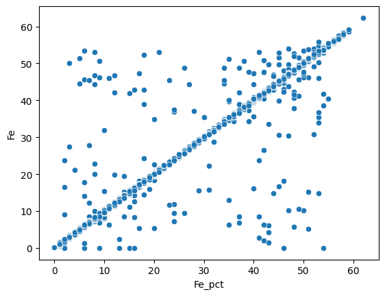
Most of the measures are similar for both methods. We can do the same for the Al2O3 weight percentage :
sns.scatterplot(data=assay_final, x="Al2O3_x", y="Al2O3_y");
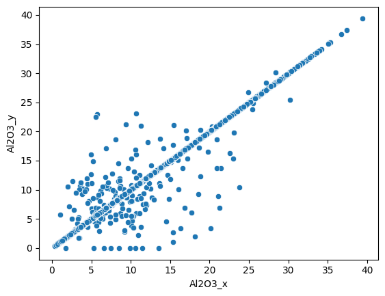
Here we also see a good correlation between the two dataset.
assay_final.drop(columns=["Al2O3_y", "LOI_x", "LOI_y"], inplace=True)
assay_final.rename(columns={"Al2O3_x": "Al2O3"}, inplace=True)
assay_final.to_csv("../data/assay_hyper.csv", index=False)