Comparison of the assay and hyperspectral datas#
The assay file contains the Hole_ID of every drill core, their position in the drill, the chemical composition of the sample (Fe, Fe2O3, P, S, SiO2, Al2O3, MnO, Mn, CaO, K2O, MgO, Na2O, TiO2) and the loss-on-ignition percentage.
The hyperspectral file contains the Hole_ID of every borehole, their position in the drill, the chemical composition of each sample (Fe, Al2O3, SiO2, K2O, CaO, MgO, TiO2, P, S, Mn), the loss-on-ignition percentage and other informations about the minerals in the sample.
The common data between these two files are the Hole_ID, the depth, most columns about chemical composition (Fe, Al2O3, SiO2, K2O, CaO, MgO, TiO2, P, S, Mn) and the loss-on-ignition percentage.
import numpy as np
import pandas as pd
import geolime as geo
from pyproj import CRS
import seaborn as sns
import pyvista as pv

pv.set_jupyter_backend('html')

geo.Logger().set_level(25)
# Format Pandas display for clarity and readability
pd.set_option("display.max_rows", 10)
pd.set_option("display.max_columns", 500)
We want to compare the Hole_ID of the assay and hyperspectral file to know if they have some drill core in common.
First we need to import these data from .csv files.
Merging Interval Files#
Assay File reading and formatting#
assay = geo.datasets.load("rocklea_dome/assay.csv")
assay
| Hole_ID | From | To | Sample_ID | Fe | Fe2o3 | P | S | SiO2 | Al2O3 | MnO | Mn | CaO | K2O | MgO | Na2O | TiO2 | LOI | LOI_100 | |
|---|---|---|---|---|---|---|---|---|---|---|---|---|---|---|---|---|---|---|---|
| 0 | RKC001 | 35.0 | 36.0 | 36.0 | 0.0 | 0 | 0 | 0 | 0.0 | 0.0 | 0.0 | 0.0 | 0.0 | 0.0 | 0.0 | 0.0 | 0 | 0 | 0.0 |
| 1 | RKC001 | 36.0 | 37.0 | 37.0 | 0.0 | 0 | 0 | 0 | 0.0 | 0.0 | 0.0 | 0.0 | 0.0 | 0.0 | 0.0 | 0.0 | 0 | 0 | 0.0 |
| 2 | RKC001 | 37.0 | 38.0 | 38.0 | 0.0 | 0 | 0 | 0 | 0.0 | 0.0 | 0.0 | 0.0 | 0.0 | 0.0 | 0.0 | 0.0 | 0 | 0 | 0.0 |
| 3 | RKC001 | 38.0 | 39.0 | 39.0 | 0.0 | 0 | 0 | 0 | 0.0 | 0.0 | 0.0 | 0.0 | 0.0 | 0.0 | 0.0 | 0.0 | 0 | 0 | 0.0 |
| 4 | RKC001 | 39.0 | 40.0 | 40.0 | 0.0 | 0 | 0 | 0 | 0.0 | 0.0 | 0.0 | 0.0 | 0.0 | 0.0 | 0.0 | 0.0 | 0 | 0 | 0.0 |
| ... | ... | ... | ... | ... | ... | ... | ... | ... | ... | ... | ... | ... | ... | ... | ... | ... | ... | ... | ... |
| 17461 | RKD010 | 0.0 | 44.0 | NaN | 0.0 | 0 | 0 | 0 | 0.0 | 0.0 | 0.0 | 0.0 | 0.0 | 0.0 | 0.0 | 0.0 | 0 | 0 | 0.0 |
| 17462 | RKD011 | 0.0 | 42.5 | NaN | 0.0 | 0 | 0 | 0 | 0.0 | 0.0 | 0.0 | 0.0 | 0.0 | 0.0 | 0.0 | 0.0 | 0 | 0 | 0.0 |
| 17463 | RKD013 | 0.0 | 30.0 | NaN | 0.0 | 0 | 0 | 0 | 0.0 | 0.0 | 0.0 | 0.0 | 0.0 | 0.0 | 0.0 | 0.0 | 0 | 0 | 0.0 |
| 17464 | RKD014 | 0.0 | 44.0 | NaN | 0.0 | 0 | 0 | 0 | 0.0 | 0.0 | 0.0 | 0.0 | 0.0 | 0.0 | 0.0 | 0.0 | 0 | 0 | 0.0 |
| 17465 | RKD015 | 0.0 | 41.0 | NaN | 0.0 | 0 | 0 | 0 | 0.0 | 0.0 | 0.0 | 0.0 | 0.0 | 0.0 | 0.0 | 0.0 | 0 | 0 | 0.0 |
17466 rows × 19 columns
Some columns have string values named LNR, replacing them to NaN will allow comparisons with other number columns
assay.dtypes
Hole_ID       object
From         float64
To           float64
Sample_ID    float64
Fe           float64
              ...
MgO          float64
Na2O         float64
TiO2          object
LOI           object
LOI_100      float64
Length: 19, dtype: object
assay.eq("LNR").any()
Hole_ID      False
From         False
To           False
Sample_ID    False
Fe           False
             ...
MgO          False
Na2O         False
TiO2          True
LOI           True
LOI_100      False
Length: 19, dtype: bool
assay.replace("LNR", np.nan, inplace=True)
assay[["P", "S", "TiO2", "LOI"]] = assay[["P", "S", "TiO2", "LOI"]].apply(pd.to_numeric)
Hyperspec File reading#
hyperspec = pd.read_csv("../data/hyperspec.csv")
hyperspec
| Hole_ID | From | To | Fe_pct | Al2O3 | SiO2_pct | K2O_pct | CaO_pct | MgO_pct | TiO2_pct | P_pct | S_pct | Mn_pct | LOI | Fe_ox_ai | hem_over_goe | kaolin_abundance | kaolin_composition | wmAlsmai | wmAlsmci | carbai3pfit | carbci3pfit | |
|---|---|---|---|---|---|---|---|---|---|---|---|---|---|---|---|---|---|---|---|---|---|---|
| 0 | RKC278 | 0.0 | 1.0 | NaN | NaN | NaN | NaN | NaN | NaN | NaN | NaN | NaN | NaN | NaN | 0.1290 | 891.13 | 0.0374 | 0.999 | NaN | NaN | NaN | NaN |
| 1 | RKC278 | 1.0 | 2.0 | NaN | NaN | NaN | NaN | NaN | NaN | NaN | NaN | NaN | NaN | NaN | 0.1460 | 892.68 | 0.0269 | 1.006 | NaN | NaN | NaN | NaN |
| 2 | RKC278 | 2.0 | 3.0 | NaN | NaN | NaN | NaN | NaN | NaN | NaN | NaN | NaN | NaN | NaN | 0.1650 | 895.24 | NaN | NaN | NaN | NaN | NaN | NaN |
| 3 | RKC278 | 3.0 | 4.0 | NaN | NaN | NaN | NaN | NaN | NaN | NaN | NaN | NaN | NaN | NaN | 0.1000 | 893.34 | NaN | NaN | 0.0545 | 2211.83 | NaN | NaN |
| 4 | RKC278 | 4.0 | 5.0 | NaN | NaN | NaN | NaN | NaN | NaN | NaN | NaN | NaN | NaN | NaN | 0.0445 | 910.32 | NaN | NaN | NaN | NaN | 0.111 | 2312.89 |
| ... | ... | ... | ... | ... | ... | ... | ... | ... | ... | ... | ... | ... | ... | ... | ... | ... | ... | ... | ... | ... | ... | ... |
| 7103 | RKC485 | 41.0 | 42.0 | 28.0 | 9.80 | 39.05 | 0.037 | 0.08 | 0.22 | 1.078 | 0.027 | 0.006 | 0.12 | 9.00 | 0.2210 | 912.17 | 0.0322 | 1.004 | NaN | NaN | NaN | NaN |
| 7104 | RKC485 | 42.0 | 43.0 | 39.0 | 7.67 | 25.15 | 0.029 | 0.09 | 0.25 | 0.689 | 0.046 | 0.008 | 0.11 | 10.11 | 0.1200 | 912.43 | 0.1140 | 1.027 | NaN | NaN | NaN | NaN |
| 7105 | RKC485 | 43.0 | 44.0 | 16.0 | 20.23 | 43.41 | 0.177 | 0.17 | 0.34 | 1.617 | 0.020 | 0.018 | 0.05 | 10.80 | 0.0956 | 888.81 | 0.0306 | 1.012 | NaN | NaN | NaN | NaN |
| 7106 | RKC485 | 44.0 | 45.0 | 12.0 | 12.53 | 50.24 | 0.060 | 0.26 | 0.25 | 1.473 | 0.006 | 0.779 | 0.03 | 16.18 | 0.0378 | 958.21 | 0.1100 | 1.025 | NaN | NaN | NaN | NaN |
| 7107 | RKD015 | 0.0 | 1.0 | NaN | NaN | NaN | NaN | NaN | NaN | NaN | NaN | NaN | NaN | NaN | NaN | NaN | NaN | NaN | NaN | NaN | NaN | NaN |
7108 rows × 22 columns
Merge Preparation#
The comparison of the two datasets require to have the list of the different Hole_ID of both files. These lists also need to be turned into sets in order to compare them.
colonne_assay = set(assay["Hole_ID"])
colonne_hyperspec = set(hyperspec["Hole_ID"])
Now we have two sets with the different drill core that have been analyzed for each method.
len(colonne_assay)
500
len(colonne_hyperspec)
192
Next command will search all the Hole_ID both in the assay and hyperspec file.
intersection = colonne_assay.intersection(colonne_hyperspec)
len(intersection)
192
The intersection of these two files has the same length as the smallest set, so every Hole_ID of the hyperspectral file are in the assay.
The drill cores of the hyperspectral file are included in the assay file. Now we want to see if the common columns between these two files have the same values. First we need to filter the DataFrame of the assay file in order to keep only the Hole_ID that are in common with the hyperspectral file.
intersection = list(intersection)
filtred_assay = assay[assay["Hole_ID"].isin(intersection)]
filtred_assay
| Hole_ID | From | To | Sample_ID | Fe | Fe2o3 | P | S | SiO2 | Al2O3 | MnO | Mn | CaO | K2O | MgO | Na2O | TiO2 | LOI | LOI_100 | |
|---|---|---|---|---|---|---|---|---|---|---|---|---|---|---|---|---|---|---|---|
| 9778 | RKC278 | 0.0 | 1.0 | 10001.0 | 0.00 | 0 | 0.000 | 0.000 | 0.00 | 0.00 | 0.0 | 0.000 | 0.00 | 0.000 | 0.00 | 0.0 | 0.000 | 0.00 | 0.0 |
| 9779 | RKC278 | 1.0 | 2.0 | 10002.0 | 0.00 | 0 | 0.000 | 0.000 | 0.00 | 0.00 | 0.0 | 0.000 | 0.00 | 0.000 | 0.00 | 0.0 | 0.000 | 0.00 | 0.0 |
| 9780 | RKC278 | 2.0 | 3.0 | 10003.0 | 0.00 | 0 | 0.000 | 0.000 | 0.00 | 0.00 | 0.0 | 0.000 | 0.00 | 0.000 | 0.00 | 0.0 | 0.000 | 0.00 | 0.0 |
| 9781 | RKC278 | 3.0 | 4.0 | 10004.0 | 0.00 | 0 | 0.000 | 0.000 | 0.00 | 0.00 | 0.0 | 0.000 | 0.00 | 0.000 | 0.00 | 0.0 | 0.000 | 0.00 | 0.0 |
| 9782 | RKC278 | 4.0 | 5.0 | 10005.0 | 0.00 | 0 | 0.000 | 0.000 | 0.00 | 0.00 | 0.0 | 0.000 | 0.00 | 0.000 | 0.00 | 0.0 | 0.000 | 0.00 | 0.0 |
| ... | ... | ... | ... | ... | ... | ... | ... | ... | ... | ... | ... | ... | ... | ... | ... | ... | ... | ... | ... |
| 17379 | RKC485 | 13.0 | 14.0 | 17215.0 | 10.73 | 0 | 0.003 | 0.021 | 48.30 | 21.94 | 0.0 | 0.001 | 0.92 | 0.055 | 2.04 | 0.0 | 1.379 | 9.84 | 0.0 |
| 17380 | RKC485 | 10.0 | 11.0 | 17212.0 | 11.74 | 0 | 0.005 | 0.023 | 46.01 | 19.45 | 0.0 | 0.001 | 2.23 | 0.063 | 2.39 | 0.0 | 1.699 | 10.59 | 0.0 |
| 17381 | RKC485 | 11.0 | 12.0 | 17213.0 | 11.25 | 0 | 0.002 | 0.010 | 48.25 | 18.76 | 0.0 | 0.001 | 1.84 | 0.054 | 2.49 | 0.0 | 1.407 | 9.92 | 0.0 |
| 17382 | RKC485 | 12.0 | 13.0 | 17214.0 | 8.41 | 0 | 0.001 | 0.007 | 49.28 | 19.61 | 0.0 | 0.001 | 3.75 | 0.058 | 2.58 | 0.0 | 1.239 | 11.19 | 0.0 |
| 17465 | RKD015 | 0.0 | 41.0 | NaN | 0.00 | 0 | 0.000 | 0.000 | 0.00 | 0.00 | 0.0 | 0.000 | 0.00 | 0.000 | 0.00 | 0.0 | 0.000 | 0.00 | 0.0 |
7235 rows × 19 columns
The next operation will delete every sample of the assay file that is not in the hyperspectral file and make sure that we have the exact same number of Hole_ID in both files.
assay_final = hyperspec.merge(filtred_assay, on=["Hole_ID", "From", "To"], how="left")
assay_final.sort_values(by=["Hole_ID", "From"], inplace=True)
assay_final
| Hole_ID | From | To | Fe_pct | Al2O3_x | SiO2_pct | K2O_pct | CaO_pct | MgO_pct | TiO2_pct | P_pct | S_pct | Mn_pct | LOI_x | Fe_ox_ai | hem_over_goe | kaolin_abundance | kaolin_composition | wmAlsmai | wmAlsmci | carbai3pfit | carbci3pfit | Sample_ID | Fe | Fe2o3 | P | S | SiO2 | Al2O3_y | MnO | Mn | CaO | K2O | MgO | Na2O | TiO2 | LOI_y | LOI_100 | |
|---|---|---|---|---|---|---|---|---|---|---|---|---|---|---|---|---|---|---|---|---|---|---|---|---|---|---|---|---|---|---|---|---|---|---|---|---|---|---|
| 0 | RKC278 | 0.0 | 1.0 | NaN | NaN | NaN | NaN | NaN | NaN | NaN | NaN | NaN | NaN | NaN | 0.1290 | 891.13 | 0.0374 | 0.999 | NaN | NaN | NaN | NaN | 10001.0 | 0.00 | 0.0 | 0.000 | 0.000 | 0.00 | 0.00 | 0.0 | 0.00 | 0.00 | 0.000 | 0.00 | 0.0 | 0.000 | 0.00 | 0.0 |
| 1 | RKC278 | 1.0 | 2.0 | NaN | NaN | NaN | NaN | NaN | NaN | NaN | NaN | NaN | NaN | NaN | 0.1460 | 892.68 | 0.0269 | 1.006 | NaN | NaN | NaN | NaN | 10002.0 | 0.00 | 0.0 | 0.000 | 0.000 | 0.00 | 0.00 | 0.0 | 0.00 | 0.00 | 0.000 | 0.00 | 0.0 | 0.000 | 0.00 | 0.0 |
| 2 | RKC278 | 2.0 | 3.0 | NaN | NaN | NaN | NaN | NaN | NaN | NaN | NaN | NaN | NaN | NaN | 0.1650 | 895.24 | NaN | NaN | NaN | NaN | NaN | NaN | 10003.0 | 0.00 | 0.0 | 0.000 | 0.000 | 0.00 | 0.00 | 0.0 | 0.00 | 0.00 | 0.000 | 0.00 | 0.0 | 0.000 | 0.00 | 0.0 |
| 3 | RKC278 | 3.0 | 4.0 | NaN | NaN | NaN | NaN | NaN | NaN | NaN | NaN | NaN | NaN | NaN | 0.1000 | 893.34 | NaN | NaN | 0.0545 | 2211.83 | NaN | NaN | 10004.0 | 0.00 | 0.0 | 0.000 | 0.000 | 0.00 | 0.00 | 0.0 | 0.00 | 0.00 | 0.000 | 0.00 | 0.0 | 0.000 | 0.00 | 0.0 |
| 4 | RKC278 | 4.0 | 5.0 | NaN | NaN | NaN | NaN | NaN | NaN | NaN | NaN | NaN | NaN | NaN | 0.0445 | 910.32 | NaN | NaN | NaN | NaN | 0.111 | 2312.89 | 10005.0 | 0.00 | 0.0 | 0.000 | 0.000 | 0.00 | 0.00 | 0.0 | 0.00 | 0.00 | 0.000 | 0.00 | 0.0 | 0.000 | 0.00 | 0.0 |
| ... | ... | ... | ... | ... | ... | ... | ... | ... | ... | ... | ... | ... | ... | ... | ... | ... | ... | ... | ... | ... | ... | ... | ... | ... | ... | ... | ... | ... | ... | ... | ... | ... | ... | ... | ... | ... | ... | ... |
| 7103 | RKC485 | 41.0 | 42.0 | 28.0 | 9.80 | 39.05 | 0.037 | 0.08 | 0.22 | 1.078 | 0.027 | 0.006 | 0.12 | 9.00 | 0.2210 | 912.17 | 0.0322 | 1.004 | NaN | NaN | NaN | NaN | 17244.0 | 28.01 | 0.0 | 0.027 | 0.006 | 39.05 | 9.80 | 0.0 | 0.12 | 0.08 | 0.037 | 0.22 | 0.0 | 1.078 | 9.00 | 0.0 |
| 7104 | RKC485 | 42.0 | 43.0 | 39.0 | 7.67 | 25.15 | 0.029 | 0.09 | 0.25 | 0.689 | 0.046 | 0.008 | 0.11 | 10.11 | 0.1200 | 912.43 | 0.1140 | 1.027 | NaN | NaN | NaN | NaN | 17245.0 | 38.60 | 0.0 | 0.046 | 0.008 | 25.15 | 7.67 | 0.0 | 0.11 | 0.09 | 0.029 | 0.25 | 0.0 | 0.689 | 10.11 | 0.0 |
| 7105 | RKC485 | 43.0 | 44.0 | 16.0 | 20.23 | 43.41 | 0.177 | 0.17 | 0.34 | 1.617 | 0.020 | 0.018 | 0.05 | 10.80 | 0.0956 | 888.81 | 0.0306 | 1.012 | NaN | NaN | NaN | NaN | 17246.0 | 15.53 | 0.0 | 0.020 | 0.018 | 43.41 | 20.23 | 0.0 | 0.05 | 0.17 | 0.177 | 0.34 | 0.0 | 1.617 | 10.80 | 0.0 |
| 7106 | RKC485 | 44.0 | 45.0 | 12.0 | 12.53 | 50.24 | 0.060 | 0.26 | 0.25 | 1.473 | 0.006 | 0.779 | 0.03 | 16.18 | 0.0378 | 958.21 | 0.1100 | 1.025 | NaN | NaN | NaN | NaN | 17247.0 | 12.22 | 0.0 | 0.006 | 0.779 | 50.24 | 12.53 | 0.0 | 0.03 | 0.26 | 0.060 | 0.25 | 0.0 | 1.473 | 16.18 | 0.0 |
| 7107 | RKD015 | 0.0 | 1.0 | NaN | NaN | NaN | NaN | NaN | NaN | NaN | NaN | NaN | NaN | NaN | NaN | NaN | NaN | NaN | NaN | NaN | NaN | NaN | NaN | NaN | NaN | NaN | NaN | NaN | NaN | NaN | NaN | NaN | NaN | NaN | NaN | NaN | NaN | NaN |
7108 rows × 38 columns
Merged Data Verification#
This new file allows to make comparison between the data from the assay file (obtain by a XRF analysis) and the data from the hyperspectral analysis.
First we can compare the Fe weight percentage :
sns.scatterplot(data=assay_final, x="Fe", y="Fe_pct");
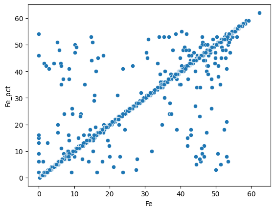
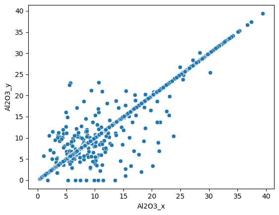
Most of the measures are similar for both methods. We can do the same for the Al2O3 weight percentage :
sns.scatterplot(data=assay_final, x="Al2O3_x", y="Al2O3_y");
assay_final.drop(columns=["Al2O3_y", "LOI_x", "LOI_y"], inplace=True)
assay_final.rename(columns={"Al2O3_x": "Al2O3"}, inplace=True)
GeoLime Drillholes Creation#
The next command will use the Geo Lime dictionary to draw an interactive map of the ferric concentration for each method (one for the hyperspectral datas and one for the assay datas). Firs we need to import the survey and collar file to have all the informations about the drill cores.
survey = geo.datasets.load("rocklea_dome/survey.csv")
collar = geo.datasets.load("rocklea_dome/collar.csv")
Project Definition#
geo.Project().set_crs(CRS("EPSG:20350"))
Drillholes Creation#
Using Assay Data Only#
da = geo.create_drillholes(
    name="rck_assay",
    collar=collar,
    assays=assay,
    survey=survey
)
da.describe()
| __TOPO_LEVEL__ | __TOPO_TYPE__ | __TOPO_ELEMENT_V1__ | __TOPO_ELEMENT_V2__ | FROM | TO | X_COLLAR | Y_COLLAR | Z_COLLAR | X_M | Y_M | Z_M | X_B | Y_B | Z_B | X_E | Y_E | Z_E | Sample_ID | Fe | Fe2o3 | P | S | SiO2 | Al2O3 | MnO | Mn | CaO | K2O | MgO | Na2O | TiO2 | LOI | LOI_100 | Depth | |
|---|---|---|---|---|---|---|---|---|---|---|---|---|---|---|---|---|---|---|---|---|---|---|---|---|---|---|---|---|---|---|---|---|---|---|---|
| count | 17466.0 | 17466.0 | 17466.000000 | 17466.000000 | 17466.000000 | 17466.000000 | 17466.000000 | 1.746600e+04 | 17466.000000 | 17466.000000 | 1.746600e+04 | 17466.000000 | 17466.000000 | 1.746600e+04 | 17466.000000 | 17466.000000 | 1.746600e+04 | 17466.000000 | 15061.000000 | 17466.000000 | 17466.0 | 16797.000000 | 16796.000000 | 17466.000000 | 17466.000000 | 17466.000000 | 17466.000000 | 17466.000000 | 17466.000000 | 17466.000000 | 17466.000000 | 17465.000000 | 17459.000000 | 17466.000000 | 17466.000000 |
| mean | 2.0 | 1.0 | 8974.469655 | 8975.469655 | 20.102900 | 21.138741 | 543919.388074 | 7.475144e+06 | 448.434576 | 543919.388074 | 7.475144e+06 | 427.813755 | 543919.388074 | 7.475144e+06 | 428.331676 | 543919.388074 | 7.475144e+06 | 427.295835 | 8460.010026 | 20.829760 | 0.0 | 0.014703 | 0.048990 | 20.605162 | 7.200063 | 0.002967 | 0.061429 | 1.049226 | 0.127557 | 0.853192 | 0.000698 | 0.418751 | 8.261108 | 8.390285 | 41.334051 |
| std | 0.0 | 0.0 | 5187.058469 | 5187.058469 | 14.265524 | 14.271989 | 5989.064771 | 1.926010e+03 | 18.584016 | 5989.064771 | 1.926010e+03 | 20.738886 | 5989.064771 | 1.926010e+03 | 20.750207 | 5989.064771 | 1.926010e+03 | 20.736974 | 5088.312571 | 20.344777 | 0.0 | 0.025723 | 0.346264 | 22.467024 | 7.547804 | 0.392103 | 0.146773 | 3.343146 | 0.460913 | 1.828060 | 0.072275 | 0.514699 | 93.754093 | 26.125344 | 13.671429 |
| min | 2.0 | 1.0 | 0.000000 | 1.000000 | 0.000000 | 1.000000 | 525400.000000 | 7.469518e+06 | 385.900000 | 525400.000000 | 7.469518e+06 | 362.600000 | 525400.000000 | 7.469518e+06 | 363.100000 | 525400.000000 | 7.469518e+06 | 362.100000 | -8888.000000 | 0.000000 | 0.0 | 0.000000 | 0.000000 | 0.000000 | 0.000000 | 0.000000 | 0.000000 | 0.000000 | 0.000000 | 0.000000 | 0.000000 | 0.000000 | 0.000000 | 0.000000 | 7.000000 |
| 25% | 2.0 | 1.0 | 4486.250000 | 4487.250000 | 9.000000 | 10.000000 | 540200.000000 | 7.473600e+06 | 440.000000 | 540200.000000 | 7.473600e+06 | 413.200000 | 540200.000000 | 7.473600e+06 | 413.700000 | 540200.000000 | 7.473600e+06 | 412.700000 | 3979.000000 | 0.000000 | 0.0 | 0.000000 | 0.000000 | 0.000000 | 0.000000 | 0.000000 | 0.000000 | 0.000000 | 0.000000 | 0.000000 | 0.000000 | 0.000000 | 0.000000 | 0.000000 | 31.000000 |
| 50% | 2.0 | 1.0 | 8971.500000 | 8972.500000 | 18.000000 | 19.000000 | 547197.500000 | 7.475598e+06 | 454.100000 | 547197.500000 | 7.475598e+06 | 429.700000 | 547197.500000 | 7.475598e+06 | 430.200000 | 547197.500000 | 7.475598e+06 | 429.100000 | 8043.000000 | 14.595000 | 0.0 | 0.005000 | 0.006000 | 12.370000 | 5.520000 | 0.000000 | 0.010000 | 0.100000 | 0.025000 | 0.290000 | 0.000000 | 0.241000 | 9.320000 | 0.000000 | 43.000000 |
| 75% | 2.0 | 1.0 | 13465.500000 | 13466.500000 | 29.000000 | 30.000000 | 547900.500000 | 7.476399e+06 | 461.700000 | 547900.500000 | 7.476399e+06 | 443.800000 | 547900.500000 | 7.476399e+06 | 444.400000 | 547900.500000 | 7.476399e+06 | 443.300000 | 12941.000000 | 41.250000 | 0.0 | 0.024000 | 0.020000 | 35.400000 | 11.550000 | 0.000000 | 0.090000 | 0.320000 | 0.095000 | 0.750000 | 0.000000 | 0.650000 | 11.550000 | 0.000000 | 49.000000 |
| max | 2.0 | 1.0 | 17964.000000 | 17965.000000 | 108.000000 | 109.000000 | 549297.900000 | 7.479595e+06 | 478.600000 | 549297.900000 | 7.479595e+06 | 478.100000 | 549297.900000 | 7.479595e+06 | 478.600000 | 549297.900000 | 7.479595e+06 | 477.600000 | 17330.000000 | 62.340000 | 0.0 | 0.845000 | 14.145000 | 96.360000 | 39.430000 | 51.820000 | 6.370000 | 40.820000 | 21.250000 | 20.010000 | 9.000000 | 10.000000 | 12367.000000 | 100.000000 | 109.000000 |
da.plot_2d(property="Fe", agg_method="mean", interactive_map=True)
Using Merged Data (Assay data & Hyperspectral data)#
df = geo.create_drillholes(
    name="rck_assay_final",
    collar=collar,
    assays=assay_final,
    survey=survey
)
df.to_file("../data/dh_hyper")
df.plot_2d(property="Fe", agg_method="mean", interactive_map=True)
Using Hyperspectral Data only#
We can do the same with hyperspectral data and draw the map of the average iron weight concentration given by these measures.
dh = geo.create_drillholes(
    name="rck_hs",
    collar=collar,
    assays=hyperspec,
    survey=survey
)
dh.describe()
| __TOPO_LEVEL__ | __TOPO_TYPE__ | __TOPO_ELEMENT_V1__ | __TOPO_ELEMENT_V2__ | FROM | TO | X_COLLAR | Y_COLLAR | Z_COLLAR | X_M | Y_M | Z_M | X_B | Y_B | Z_B | X_E | Y_E | Z_E | Fe_pct | Al2O3 | SiO2_pct | K2O_pct | CaO_pct | MgO_pct | TiO2_pct | P_pct | S_pct | Mn_pct | LOI | Fe_ox_ai | hem_over_goe | kaolin_abundance | kaolin_composition | wmAlsmai | wmAlsmci | carbai3pfit | carbci3pfit | Depth | |
|---|---|---|---|---|---|---|---|---|---|---|---|---|---|---|---|---|---|---|---|---|---|---|---|---|---|---|---|---|---|---|---|---|---|---|---|---|---|---|
| count | 7108.0 | 7108.0 | 7108.000000 | 7108.000000 | 7108.000000 | 7108.000000 | 7108.000000 | 7.108000e+03 | 7108.000000 | 7108.000000 | 7.108000e+03 | 7108.000000 | 7108.000000 | 7.108000e+03 | 7108.000000 | 7108.000000 | 7.108000e+03 | 7108.000000 | 4962.000000 | 4962.000000 | 4962.000000 | 4945.000000 | 4962.000000 | 4961.000000 | 4962.000000 | 4582.000000 | 4635.000000 | 3696.000000 | 4955.000000 | 6896.000000 | 6639.00000 | 3841.000000 | 3841.000000 | 1689.000000 | 1689.000000 | 343.000000 | 343.000000 | 7108.000000 |
| mean | 2.0 | 1.0 | 3649.240293 | 3650.240293 | 20.568655 | 21.568655 | 547413.687521 | 7.475481e+06 | 458.500774 | 547413.687521 | 7.475481e+06 | 437.432119 | 547413.687521 | 7.475481e+06 | 437.932119 | 547413.687521 | 7.475481e+06 | 436.932119 | 31.597340 | 10.943720 | 28.319313 | 0.181180 | 1.501790 | 1.254634 | 0.631873 | 0.027161 | 0.054300 | 0.109976 | 11.297941 | 0.175376 | 910.74075 | 0.162194 | 1.023886 | 0.053203 | 2207.762297 | 0.070173 | 2319.090816 | 42.645751 |
| std | 0.0 | 0.0 | 2111.443717 | 2111.443717 | 13.834178 | 13.834178 | 685.729896 | 1.587386e+03 | 7.467718 | 685.729896 | 1.587386e+03 | 15.848056 | 685.729896 | 1.587386e+03 | 15.848056 | 685.729896 | 1.587386e+03 | 15.848056 | 17.845885 | 7.396816 | 19.816311 | 0.494112 | 4.219235 | 2.269107 | 0.524281 | 0.038540 | 0.371307 | 0.165558 | 4.640690 | 0.083901 | 8.87125 | 0.082431 | 0.046539 | 0.038201 | 3.049294 | 0.024599 | 9.787246 | 11.275263 |
| min | 2.0 | 1.0 | 0.000000 | 1.000000 | 0.000000 | 1.000000 | 545494.900000 | 7.472793e+06 | 441.000000 | 545494.900000 | 7.472793e+06 | 389.700000 | 545494.900000 | 7.472793e+06 | 390.200000 | 545494.900000 | 7.472793e+06 | 389.200000 | 0.000000 | 0.320000 | 2.380000 | 0.003000 | 0.010000 | 0.020000 | 0.003000 | 0.001000 | 0.001000 | 0.010000 | 0.710000 | 0.001300 | 869.78000 | 0.017200 | 0.937000 | 0.020000 | 2186.280000 | 0.040100 | 2296.430000 | 7.000000 |
| 25% | 2.0 | 1.0 | 1816.750000 | 1817.750000 | 9.000000 | 10.000000 | 546904.700000 | 7.474003e+06 | 453.800000 | 546904.700000 | 7.474003e+06 | 425.900000 | 546904.700000 | 7.474003e+06 | 426.400000 | 546904.700000 | 7.474003e+06 | 425.400000 | 14.000000 | 5.370000 | 11.180000 | 0.022000 | 0.100000 | 0.280000 | 0.227000 | 0.009000 | 0.006000 | 0.030000 | 9.670000 | 0.107000 | 907.70000 | 0.091100 | 0.991000 | 0.028100 | 2206.370000 | 0.052750 | 2312.235000 | 36.000000 |
| 50% | 2.0 | 1.0 | 3650.500000 | 3651.500000 | 19.000000 | 20.000000 | 547586.100000 | 7.475604e+06 | 458.200000 | 547586.100000 | 7.475604e+06 | 439.000000 | 547586.100000 | 7.475604e+06 | 439.500000 | 547586.100000 | 7.475604e+06 | 438.500000 | 35.000000 | 8.880000 | 22.660000 | 0.049000 | 0.190000 | 0.480000 | 0.484000 | 0.021000 | 0.013000 | 0.080000 | 11.200000 | 0.185000 | 911.14000 | 0.161000 | 1.007000 | 0.039600 | 2206.910000 | 0.063600 | 2321.900000 | 46.000000 |
| 75% | 2.0 | 1.0 | 5479.250000 | 5480.250000 | 31.000000 | 32.000000 | 547947.600000 | 7.476004e+06 | 463.600000 | 547947.600000 | 7.476004e+06 | 449.500000 | 547947.600000 | 7.476004e+06 | 450.000000 | 547947.600000 | 7.476004e+06 | 449.000000 | 48.000000 | 15.255000 | 42.560000 | 0.137000 | 0.500000 | 1.020000 | 0.897000 | 0.036000 | 0.025000 | 0.150000 | 11.900000 | 0.246000 | 914.48000 | 0.226000 | 1.050000 | 0.064300 | 2208.140000 | 0.080500 | 2324.615000 | 51.000000 |
| max | 2.0 | 1.0 | 7298.000000 | 7299.000000 | 60.000000 | 61.000000 | 548498.100000 | 7.479595e+06 | 478.600000 | 548498.100000 | 7.479595e+06 | 478.100000 | 548498.100000 | 7.479595e+06 | 478.600000 | 548498.100000 | 7.479595e+06 | 477.600000 | 62.000000 | 39.430000 | 92.810000 | 9.504000 | 40.820000 | 20.010000 | 3.742000 | 0.845000 | 14.145000 | 6.160000 | 45.280000 | 0.355000 | 974.08000 | 0.413000 | 1.192000 | 0.285000 | 2233.120000 | 0.182000 | 2338.390000 | 61.000000 |
dh.plot_2d(property="Fe_pct", agg_method="mean", interactive_map=True)
The first thing we can notice is that there is a concentration of high average iron concentration in the eastern drill core of the original assay data. That is on those drill core that the hyperspectral data have been taken. Then we can also notice the strong similarity between the iron average concentration between the hyperspectral data and the assay data for the same drill holes.
3D Visualisation#
df_pv = df.to_pyvista('Fe_pct')
pl = pv.Plotter()
pl.add_mesh(df_pv.tube(radius=10))
pl.set_scale(zscale=20)

pl.show()