Variography

import geolime as geo

dh_tom = geo.read_file("../data/dh_tom_comp.geo")

Once the capping value determined, we can create a new property to capp the value above 25.

dh_tom.set_property(name='Zn_cap', data='Zn_pct')
dh_tom.update_property(name='Zn_cap', data='25', region="(Zn_cap > 25)")

Normal Score

For simplicity in variography analysis, let’s compute the normal scores of the data.

gauss_score function returns a numpy array, so let’s create a new property on the Drillholes.

geo.gauss_score(dh_tom['Zn_cap'])

2026-09-22 14:28:55,052 [WARNING] GeoLime Project - |GEOLIME|.anamorphosis.py : There are NaN in data. They will be ignored.

array([-0.78162595,         nan,         nan, ..., -0.7347981 ,
       -0.97560843, -1.06290788])

dh_tom.set_property(name="Zn_gauss", data=geo.gauss_score(dh_tom['Zn_cap']))

2026-09-22 14:28:55,262 [WARNING] GeoLime Project - |GEOLIME|.anamorphosis.py : There are NaN in data. They will be ignored.

Experimental Analysis

Lag Creation

For Variography analysis, lag creation can be perfom

• implicitly with a number of lags and a length of lag

• explicitly with interval values provided.

lags, tol = geo.generate_lags_from_interval([[0, 10], [10, 20], [20, 40]])

lags, tol = geo.generate_lags(lag=40, plag=50, nlags=15)

lags

array([  0.,  40.,  80., 120., 160., 200., 240., 280., 320., 360., 400.,
       440., 480., 520., 560.])

tol

20.0

Variography Analysis is perform in 2 step:

• finding the main direction

• computing the semi variogram 1D in the major/semi-major/minor directions

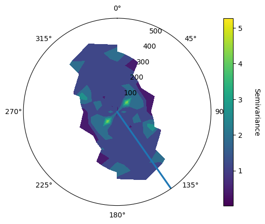
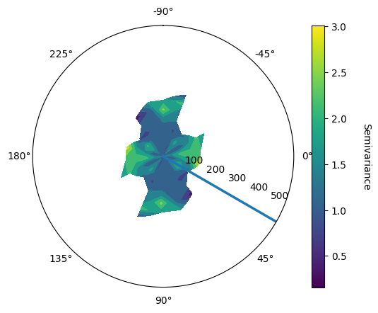
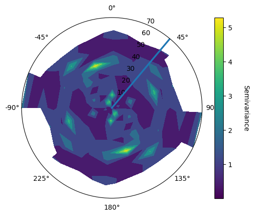
The finding of the main direction is perform through the analysis of variomap is the different planes.

• Analysis around the Z axis for the azimuth using vario_map / vario_contour;

• Once found the main azimuth, analysis around the X axis for the dip using vario_contour_dip;

• Once found the correspond azimuth and dip, analysis around the Z axis for the pitch using vario_contour_pitch

Finding main direction

geo.vario_map(
    geo_object=dh_tom,
    attribute="Zn_gauss",
    region="Zn_gauss.notna()",
    lags=lags,
    tol=tol,
    n_az=15,
    atol=15,
    backend=geo.GeostatsBackend.RUST,
    rust_multithread=True
)

geo.vario_contour(
    geo_object=dh_tom,
    attribute="Zn_gauss",
    region="Zn_gauss.notna()",
    lags=lags,
    tol=tol,
    n_az=15,
    atol=10,
    user_azimuth=145,
    backend=geo.GeostatsBackend.RUST,
    rust_multithread=True
)

geo.vario_contour_dip(
    geo_object=dh_tom,
    attribute="Zn_gauss",
    region="Zn_gauss.notna()",
    lags=lags,
    tol=tol,
    azimuth=145,
    n_dip=18,
    atol=10,
    user_dip=30,
    c_step=None,
    save_file=None,
    backend=geo.GeostatsBackend.RUST,
    rust_multithread=True
)

lags, tol = geo.generate_lags(lag=5, plag=50, nlags=15)

geo.vario_contour_pitch(
    geo_object=dh_tom,
    attribute="Zn_gauss",
    region="Zn_gauss.notna()",
    lags=lags,
    tol=tol,
    azimuth=145,
    dip=30,
    n_pitch=15,
    atol=10,
    user_pitch=40,
    c_step=None,
    save_file=None,
    backend=geo.GeostatsBackend.RUST,
    rust_multithread=True
)

Computing Major/Semi-major/minor 1D variograms

lags, tol = geo.generate_lags(lag=40, plag=50, nlags=15)

vario_exp_major = geo.variogram(
    object=dh_tom,
    attribute="Zn_gauss",
    region="Zn_gauss.notna()",
    geographic_azimuth=145,
    dip=30,
    pitch=40,
    lags=lags,
    tol=tol,
    atol=15
)

vario_exp_major

	lag	npairs	avgdist	vario
0	0.0	77.0	7.075251	0.465454
1	40.0	3398.0	40.792308	0.777678
2	80.0	40960.0	78.978592	0.806472
3	120.0	30229.0	124.929092	0.989965
4	160.0	40946.0	156.139283	1.114601
5	200.0	36114.0	203.021025	1.081230
6	240.0	25212.0	236.429496	1.037848
7	280.0	33931.0	281.395056	0.942480
8	320.0	37389.0	321.037288	1.039325
9	360.0	25154.0	358.375446	0.779454
10	400.0	26566.0	400.089684	0.820185
11	440.0	23764.0	437.470476	0.803399
12	480.0	16475.0	482.005252	0.954414
13	520.0	15733.0	520.853958	0.870195
14	560.0	15399.0	559.317753	0.754322

geo.plot_semivariogram(
    variograms=[vario_exp_major],
    display_npairs=True
)

vario_exp_semi_major = geo.variogram(
    object=dh_tom,
    attribute="Zn_gauss",
    region="Zn_gauss.notna()",
    geographic_azimuth=145,
    dip=30,
    pitch=-50,
    lags=lags,
    tol=tol,
    atol=15
)

geo.plot_semivariogram(
    variograms=[vario_exp_semi_major],
    display_npairs=True
)

lags, tol = geo.generate_lags(lag=2, plag=50, nlags=15)

vario_exp_minor = geo.variogram(
    object=dh_tom,
    attribute="Zn_gauss",
    region="Zn_gauss.notna()",
    geographic_azimuth=145,
    dip=-60,
    pitch=40,
    lags=lags,
    tol=tol,
    atol=30
)

geo.plot_semivariogram(
    variograms=[vario_exp_minor],
    display_npairs=True
)

Computing Downhole Variogram

lags, tol = geo.generate_lags(lag=1., plag=50, nlags=20)

vario_exp_bh = geo.variogram_downhole(
    object= dh_tom,
    attribute="Zn_gauss",
    region="Zn_gauss.notna()",
    lags=lags,
    tol=tol,
)

geo.plot_semivariogram(
    variograms=[vario_exp_bh],
    display_npairs=True
)

Automatic Fitting

Automatic Fitting uses an empty model to fit along experimental variograms. Fitting is usually performed in 2 steps : first fit the nugget and then fit the other structures.

Fitting the Nugget

nugget_model = geo.Nugget() + geo.Spherical()

The fitting algorithm can be set up to preferrentially fit the small ranges using the INVERSE_DISTANCE or SQUARED_INVERSE_DISTANCE.

geo.model_fit(
    variograms=[vario_exp_bh],
    cov=nugget_model,
    weighting_method=geo.VarioFitWeightingMethod.SQUARED_INVERSE_DISTANCE
)

print(nugget_model)

Model with 2 components 
 
Component 1 : 
Sill : 0.027849223671814367 
Covariance type : Nugget 

Component 2 : 
Sill : 0.6723208800070047 
Covariance type : Spherical 
Scales : (18.948289181596092, 4.749999999999999, 6.534143242414088) 
Angles : (27.8897996451133, 1e-10, 0.0) 

Total sill = 0.7001701036788192 

Model and experimental variogram can be plotted on the same graphic by specifying the parameter model and model_angles. Note that for downhole varigram the model_angles values do not have any importance.

geo.plot_semivariogram(
    variograms=[vario_exp_bh],
    model=nugget_model,
    model_angles=[{"azi":0, "dip":90, "pitch":90}],
    display_npairs=True
)

Each structure component can be accessed using the cov_elem_list attribute.

nugget_model.cov_elem_list[0].sill

0.027849223671814367

Fitting the structures

model =  geo.Nugget() + geo.Spherical() + geo.Spherical()

short_range_spherical_ratio = 0.6
long_range_spherical_ratio = 0.4

geo.model_fit(
    variograms=[
        vario_exp_major,
        vario_exp_semi_major,
        vario_exp_minor
    ],
    cov=model,
    constraints=[
        {"sill_fixed":0.13},
        {
            "sill_max": short_range_spherical_ratio * (vario_exp_major.attrs["variable_var"] - 0.13),
            "angle_fixed_0": 145,
            "angle_fixed_1": 60,
            "angle_fixed_2": 40,
            "scale_max_0":100,
            "scale_max_1":100,
            "scale_max_2":20 
        },
        {
            "sill_max": long_range_spherical_ratio * (vario_exp_major.attrs["variable_var"] - 0.13),
            "angle_fixed_0": 145,
            "angle_fixed_1": 60,
            "angle_fixed_2": 40, 
        }
    ]
)

geo.plot_semivariogram(
    variograms=[vario_exp_major, vario_exp_semi_major, vario_exp_minor],
    model=model,
    model_angles=[
        {"azi":145, "dip":60, "pitch":40},
        {"azi":145, "dip":60, "pitch":-50},
        {"azi":145, "dip":-30, "pitch":40},
    ],
    display_npairs=True
)

print(model)

Model with 3 components 
 
Component 1 : 
Sill : 0.13 
Covariance type : Nugget 

Component 2 : 
Sill : 0.5420507487187317 
Covariance type : Spherical 
Scales : (3.6444713668251176, 78.32334559584572, 11.041455233059162) 
Angles : (145.0, 60.0, 40.0) 

Component 3 : 
Sill : 0.3613696429567596 
Covariance type : Spherical 
Scales : (559.9946270658145, 13.99696317783461, 559.9975363496937) 
Angles : (145.0, 60.0, 40.0) 

Total sill = 1.0334203916754914 

dh_tom.to_file("../data/dh_tom_comp_capped.geo")